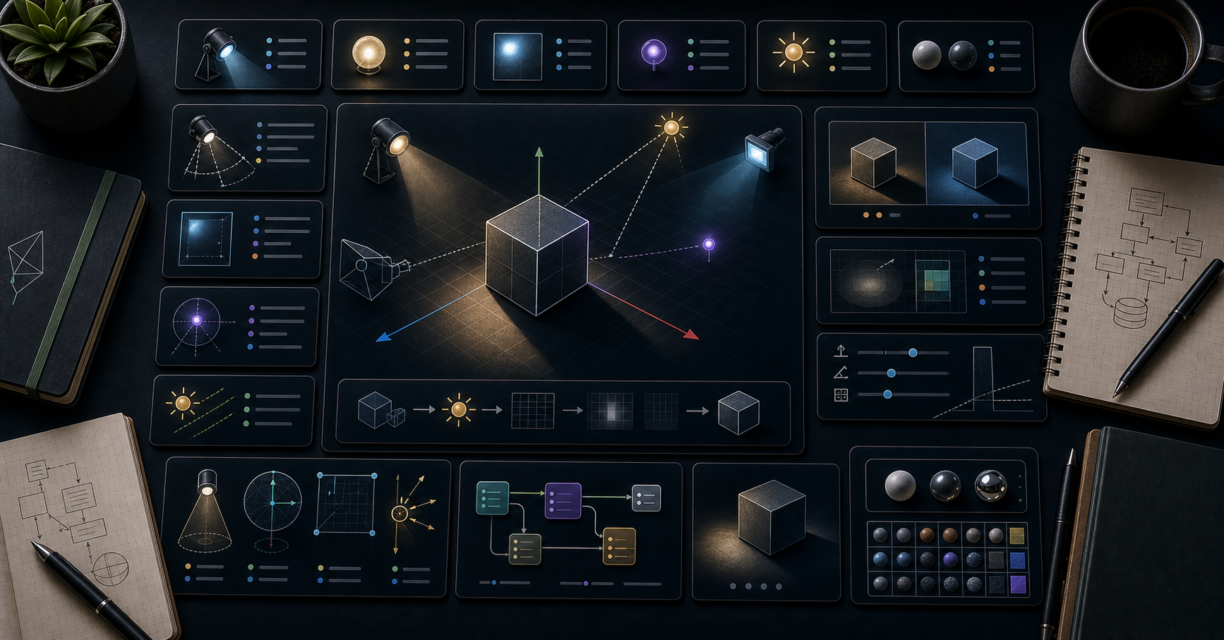
Three.js Course — 03 · Lighting & Shadows (PCF, PCFSoft, VSM, CSM, Contact)
Lighting decides whether a 3D scene looks alive or flat. Shadows decide whether objects look grounded or floating. Three.js ships six light types, three shadow-map algorithms, an add-on for cascaded shadow maps, and several "fake" shadow techniques (contact shadow, baked AO, shadow catcher). This post covers all of them, plus the bias / map-size / camera tuning that makes shadows actually look good rather than buggy.
> Series map: 00 Foundations → 01 Geometry & Materials → 02 Cameras & Controls → 03 Lighting & Shadows (this post) → 04 Textures & PBR → 05 Asset Pipeline → 06 Animation → 07 Instancing & Batching → 08 Low-End Perf → 09 Shaders → 10 Post-Processing → 11 Physics → 12 R3F → 13 AI 3D.
Learning Outcome
- Use all six light types: , , , , , .- Enable + configure shadow maps without artefacts.- Choose between , , , .- Tune , , , , and the shadow camera frustum.- Use Cascaded Shadow Maps () for large outdoor terrains.- Pick when to use a "contact shadow" (cheap fake) or a baked AO map instead.
Chapter 1 — Light types
| Light | Direction | Cast shadow? | Cost | When ||-------|-----------|--------------|------|------|| | uniform from all directions | no | free | scene "fill" so dark sides aren't black || | sky colour above + ground colour below | no | very cheap | outdoor fill (sky → blue, ground → green) || | parallel rays (like the sun) | yes | cheap-ish | sun, key light || | omni from a single point | yes (6-face cube map) | medium | lamps, fires || | cone from a point | yes | medium | flashlights, stage lights || | rectangle (area light) | no (yet) | medium | windows, softboxes; needs init |
Intensity in 2026
Since Three.js r155, physically-correct lighting is the default. Intensity is in candela (point/spot) or lumens, and interprets it physically. A intensity of ≈ noon sun. A small for a desk lamp might be .
To opt back into the old non-physical mode (for compatibility with older tutorials):
Chapter 2 — Enabling shadows (the three-step ritual)
Shadows are off by default. Three steps to turn them on:
Forget any one of these three and you'll see no shadows.
Chapter 3 — Shadow map types
| Type | Cost | Edge quality | Notes ||------|------|--------------|-------|| | cheapest | hard, pixelated | rarely used || | medium | softer than basic, default | OK || | medium-high | much softer, blurry | good default || | high (but blurrable for free) | very soft, can light-bleed | needs + tuning |
Set globally on the renderer (above). For VSM, additionally:
VSM has a unique benefit: the blur happens in screen space, so blur radius doesn't cost more shadow-map texture. Watch for light-bleeding artefacts at corners — usually fixed by adjusting and parameters or by mixing with a tiny .
Chapter 4 — The shadow camera
A shadow-casting light renders the scene from its own viewpoint into a depth texture (the shadow map). That viewpoint is a camera — orthographic for , perspective for .
The frustum must:
- Be as small as possible while enclosing every shadow caster.- Not crop the receiving floor / walls.
If too large → wasted precision → blocky shadows. If too small → shadows fade out where the frustum ends.
> Trick: add while tuning. You see the shadow camera frustum in real time. Remove for production.
Chapter 5 — Bias, normalBias, radius, mapSize
Four knobs decide whether shadows look right or covered in stripes / floating / pixelated.
| Knob | What | Typical ||------|------|---------|| | resolution of the shadow texture | 1024 / 2048 / 4096 (powers of 2) || | offsets depth to prevent shadow acne (self-shadowing artefacts) | || | offsets along surface normal — fixes "peter panning" (shadows detached from feet) | || | softening radius (PCF / VSM) | |
Classic recipe:
Symptoms / fixes:
| Symptom | Fix ||---------|-----|| Banding / stripes on lit surfaces ("shadow acne") | increase magnitude (more negative) || Shadows detached from objects ("peter pan") | increase || Edges very pixelated | bigger (cost: GPU memory + fill rate) || Shadows fade to nothing at distance | enlarge shadow camera frustum || Light-bleeding at corners (VSM) | reduce , or fall back to PCFSoft |
Chapter 6 — Cascaded Shadow Maps (CSM)
For huge outdoor terrains, a single shadow map is either pixelated everywhere (too big a frustum) or sharp near and gone far (too small). CSM splits the camera frustum into N slices (cascades), each with its own shadow map at decreasing resolution as distance grows.
Three.js doesn't ship CSM; use three-csm (or its r3f cousin ):
Use CSM whenever the visible terrain is much larger than the camera's close-up area — landscape games, open worlds, architectural visualisations of city blocks.
Chapter 7 — Contact shadows + AO + shadow-catcher tricks
Real-time shadows aren't always needed. Cheaper effects often look better.
Contact shadow ("AccumulativeShadows" / soft ground shadow)
A pre-baked or accumulated render of the object from above, splatted onto a transparent plane under it. Looks gorgeous, costs nearly nothing per frame.
- Drei: + — a one-liner in R3F.- Vanilla: render the object N times with jittered light, composite into a render target.
Ambient occlusion (AO)
The "darkening in corners + crevices" effect that ground objects in shadow without computing every light.
Two paths:
1. Baked AO — bake in Blender / Substance, export as texture, apply via .2. Screen-space AO (SSAO) — runtime post-processing pass (Post 10).
Baked is cheaper + higher quality where the geometry is static.
Shadow catcher
A plane that only displays the shadow of objects above it (transparent everywhere else). Useful for product viewers on a transparent background:
- Drei: on a plane.- Vanilla: .
Chapter 8 — Performance budget for shadows
Shadows are often the most expensive part of a Three.js scene. Rough budget:
| Setup | Frame cost (mid-range desktop) ||-------|--------------------------------|| No shadows | 0 || 1 DirectionalLight, 1024 map, PCF | 0.5-1 ms || 1 DirectionalLight, 2048 map, PCFSoft | 1-3 ms || 1 DirectionalLight, 4096 map, VSM | 3-8 ms || 4-cascade CSM, 2048 each | 6-15 ms || PointLight shadow (6-face cube) | 3-5× a DirectionalLight || 3+ shadow-casting lights | quickly exceeds budget on mobile |
Mobile cuts these costs in half on optimistic GPUs and 3× on bad ones. Plan for ≤ 1 shadow-casting light + map on phones.
> Trick: for indoor scenes with many lights, bake the lightmap (Blender → Cycles → bake → export texture → assign as ). Static lighting becomes a texture — zero per-frame cost. Real-time lights are only used for dynamic objects.
Chapter 9 — , , and shadow update modes
Two perf flags worth knowing in the lighting context:
For mostly-static scenes (architectural visualisations), turning off and only flagging when something moves is a free speed boost.
These also help shadow rendering: the shadow camera does its own frustum culling, so meshes with stale matrices waste work.
Practice Exercises
Exercise 1 — Basic shadow setup
A cube on a plane. One DirectionalLight. Walk through the three-step ritual. Confirm a shadow appears.
Exercise 2 — Compare shadow types
Same scene, cycle through , , , . Note difference in edges + framerate.
Exercise 3 — Tune bias
Deliberately set . Observe acne. Lower to until it disappears. Then experiment with on a slanted surface.
Exercise 4 — Cascaded shadow maps
Build a 200×200 terrain (). Place 100 trees (cubes for now) on it. Compare a single 4096 shadow map vs a 4-cascade CSM. Note the close-up shadow sharpness.
Exercise 5 — Shadow catcher
Load a single product model (any GLB) on a transparent plane. Render with . The result: model + soft shadow, no ground visible.
Exercise 6 — Lightmap workflow
In Blender, build a simple room (4 walls + floor), bake AO, export the AO texture. In Three.js, load the room as GLB, attach the AO texture as . Compare with and without.
Cheat-sheet
| What | How ||------|-----|| Enable shadows | || Soft shadow type | || Cast | + || Receive | (and floor) || Shadow camera frustum | tighten via || After frustum change | || Shadow resolution | || Bias defaults | , || Debug | || Cascaded shadows | library, 2-4 cascades || Contact shadow | accumulated splat or Drei || AO | bake to for static; SSAO in post for dynamic || Static scene speedup | ; flag on change || Physically correct in 2026 | default since r155; tune intensities accordingly |
What's next
Post 04 covers textures and PBR: how to load and configure colour, normal, roughness, metallic, AO maps; the sRGB / linear colour pipeline; mipmaps + anisotropy; environment maps (IBL); and KTX2 compressed textures.
References
- Three.js docs — Lights- Three.js docs — LightShadow- three-csm — cascaded shadow maps- Mastering Shadows in Three.js (dev.to)- Shadow optimisation forum thread
> Note: this post is in progress. Planned additions: ESM (Exponential Shadow Map) plugin survey; baking lightmaps in Blender step-by-step; cubeUV reflections lighting.
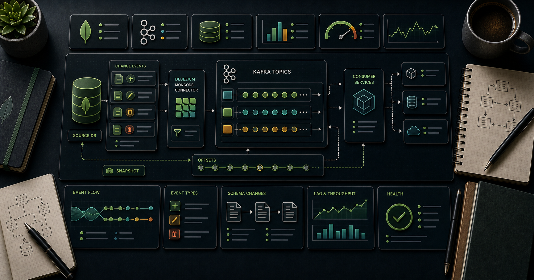
MongoDB Course — 24 · Kafka + Debezium + MongoDB Kafka Connector (Source + Sink)
The standard way to flow data between MongoDB and Kafka in 2026 is two connectors: MongoDB Kafka Source Connector (Mongo → Kafka, change-stream-based, official) and MongoDB Kafka Sink Connector (Kafka → Mongo). For cross-database CDC (Postgres → Mongo, etc.), Debezium is the de facto. This post covers all three — what each does, when to use which, configurations that work in production, deduplication + ordering, and the common pitfalls (the failed-on-update-events trap, partition keys, schema registry).
> Series map: 22 RAG → 23 SQL→Mongo migration → 24 Kafka + Debezium CDC (this post) → 25 Testing → 26 OpenTelemetry → 27 Geo → 28 Time-series extreme → 29 K8s + mongosync + cost.
Learning Outcome
- Set up Kafka + Kafka Connect locally.- Configure the MongoDB Kafka Source connector with change streams.- Configure the MongoDB Kafka Sink connector to write to a collection.- Configure Debezium Postgres connector → Kafka → Mongo sink.- Handle ordering, deduplication, schema evolution.- Recognise when to use this stack vs the simpler outbox + change-stream publisher (Post 20).
Chapter 1 — Why Kafka + Connect
Outbox + change streams (Post 20) is the cheap, self-contained pattern. Kafka + Connect earn their complexity when:
- You have many consumers for the same data (Mongo change → search index + analytics + cache + audit + downstream service).- You have multiple source DBs that should produce events in the same format (Postgres + Mongo + MySQL all into one Kafka topic family).- You need replayable storage of events for days/weeks (Kafka retention) independent of source DB oplog.- You're already on Kafka for other reasons.
If none apply, stick with Post 20. Connect adds: Kafka cluster, Schema Registry, Connect cluster, connector configs to maintain.
Chapter 2 — Architecture
Three connectors, two directions, one Kafka cluster.
Chapter 3 — MongoDB Kafka Source Connector
Reads from MongoDB change streams, publishes to Kafka topics.
Install: download the Confluent Hub connector or pull the JAR; place in Connect plugin path.
Config:
Topic name produced: ().
Key options:
- → publish only the post-image document, not the full change event envelope. Often what consumers actually want.- → fetch the post-image on update events (Post 12 Ch 4).- → on first start, snapshot the collection into Kafka before starting the change stream.- → an aggregation pipeline filter applied to events.
Apply via Connect REST API:
Chapter 4 — MongoDB Kafka Sink Connector
Reads from Kafka topics, writes to a Mongo collection.
Key options:
- — how to derive on the sink doc. Use a strategy that keys on a stable business ID (often from the source).- — how to apply each Kafka message. is upsert-by-key — idempotent, replay-safe.- + DLQ topic — bad messages don't stop the connector.
This pattern (Source → Kafka → Sink) is how you build a cross-region Mongo replica via Kafka, populate a read-model collection, or sync to another store.
Chapter 5 — Debezium MongoDB Source Connector
Debezium offers its own MongoDB source connector — equivalent to MongoDB's official Source but with the Debezium event envelope (consistent across all Debezium connectors). Pick one or the other; both work.
Default envelope:
Useful when downstream consumers want before/after + a uniform shape across Postgres + Mongo + MySQL events.
Choose MongoDB's official Source connector if you only need one direction + want simpler messages. Choose Debezium if you're standardising on its envelope.
Chapter 6 — Debezium Postgres → MongoDB Sink
The killer use case: continuously replicate Postgres tables to MongoDB without writing code.
Debezium Postgres source
Publishes one topic per table — , etc.
MongoDB Sink for Debezium events
Debezium ships a dedicated MongoDB sink connector that understands its own event envelope + handles deletes correctly. Recent versions support the standard Debezium connector pattern (every event type → matching mongo op).
> Watch out: the older MongoDB Kafka Sink (Chapter 4) doesn't natively handle Debezium update events from other DBs — you need a CDC handler () configured, and there have been update-event bugs (see references). For new Postgres→Mongo work in 2026, prefer the Debezium MongoDB sink — it's purpose-built.
Chapter 7 — Kafka topics + partitioning
For Mongo source events:
- One topic per collection (default) — easy.- Topic key = document → events for the same doc land in the same partition → preserved order per doc.
For Debezium Postgres source:
- One topic per table.- Key = primary key → ordered per row.
Partition count = expected throughput. Default 6-12 partitions per topic for medium throughput. Don't go to 100 unless you have parallel consumers to match.
Retention: 7 days default. For replay scenarios, 30 days. For Event Sourcing (Post 21), forever (compact topic or off-cluster archive).
Chapter 8 — Schema Registry + Avro / JSON Schema
Without a registry, every consumer must parse JSON heuristically + handle schema changes manually.
With Confluent Schema Registry (or Apicurio, Karapace):
- Producers register schemas.- Consumers fetch schema by ID embedded in each message.- Compatibility rules enforced (backward, forward, full).
Format choice: Avro (binary, compact, strong typing) for high-volume; JSON Schema (human-readable, debuggable) for moderate. Avro is the Kafka native; JSON Schema gaining ground.
Connectors support both. Configure once; downstream consumers get type safety + evolution rules for free.
Chapter 9 — Deduplication + ordering — same rules as outbox
Kafka delivers at-least-once (default). Consumers must be idempotent.
Patterns:
- Key by business ID → idempotent upserts at the sink.- Optimistic versioning — sink rejects events with .- Tombstone records for deletes (key = ID, value = null) — compaction-friendly.
Ordering:
- Within a partition: guaranteed.- Across partitions: not guaranteed.- Key your events so all events for one entity land in one partition.
Chapter 10 — Local dev environment
:
holds the downloaded connector JARs (Mongo source/sink + Debezium Postgres). is the friendly path.
After , hit for Connect REST. POST connector configs as in Chapters 3-6.
Chapter 11 — Production operations
- Connect cluster in distributed mode (multiple Connect workers) for HA + scalability.- Monitoring: JMX → Prometheus exporter → Grafana. Watch connector lag + DLQ size.- Backups: Connect stores state in Kafka topics — back them up.- Schema changes: register new schema versions; downstream consumers handle gracefully.- Failover: source connector resumes from stored offset on restart.- Atlas: hosted Confluent Cloud + Atlas Source/Sink work seamlessly. Many teams pick this combo for zero ops.
Chapter 12 — Comparison table
| | Outbox + change-stream (Post 20) | Mongo Source/Sink | Debezium + Sink ||---|---|---|---|| Setup complexity | minimal | medium (Kafka + Connect) | medium-high (Kafka + Connect + Debezium) || Cross-DB CDC | no | no | yes (Postgres / MySQL / etc) || Replay window | as long as you keep rows | Kafka retention (7-90 days) | Kafka retention || Event envelope | yours | Mongo's | Debezium's (consistent across DBs) || Multi-consumer fan-out | possible but custom | natural via Kafka | natural via Kafka || Cost | tiny | Kafka + Connect | Kafka + Connect |
Pick the cheapest pattern that fits the requirement.
Chapter 13 — Common pitfalls
| Pitfall | Cause | Fix ||---------|-------|-----|| Mongo Sink fails on update from Debezium | CDC handler config missing | use Debezium MongoDB sink instead, or configure || Update events arrive without | source not set | set to || Out-of-order events | partition key not on business ID | re-key || Connector lag grows | sink slow | scale sink concurrency; partition more || Schema change breaks consumers | no Schema Registry | adopt; enforce compatibility || DLQ topic ignored | no alerts on DLQ size | alert when DLQ count > 0 || Connect single-node failure | not running in distributed mode | run ≥ 2 workers || Source replicates everything (huge load) | no filter | filter event stream at source || Tombstone confusion | deletes received as null | configure handler || Debezium PG sequence reset / re-init | snapshot mode misconfigured | review |
Practice Exercises
Exercise 1 — Local stack
Stand up the from Chapter 10. Confirm Kafka, Connect, Mongo (replica set), Postgres all run.
Exercise 2 — Mongo Source
Configure the Mongo Source connector for a collection. Insert into Mongo; consume the topic with .
Exercise 3 — Mongo Sink
Add a Mongo Sink consuming the topic into . Insert into source; verify it appears in the sink within seconds.
Exercise 4 — Debezium Postgres → Mongo
Configure Debezium Postgres source + MongoDB sink. Insert into a Postgres table; verify the document appears in Mongo.
Exercise 5 — Filter at source
Add a filter to the Mongo Source connector — only events with . Confirm filter works.
Exercise 6 — DLQ
Misconfigure a sink (wrong field type). Send a bad message; confirm it lands in the DLQ topic instead of stopping the connector.
Cheat-sheet
| What | How ||------|-----|| Mongo → Kafka | MongoDB Kafka Source connector (official) || Kafka → Mongo | MongoDB Kafka Sink connector || Postgres → Mongo | Debezium PG source + Debezium MongoDB sink || Mongo → other DB | MongoDB Source + that DB's sink || Full doc on update | || Publish post-image only | || Snapshot on first run | || Idempotent sink | on || Error policy | + DLQ topic || Schema | use Schema Registry (Avro / JSON Schema) || Order per entity | key on business ID → same partition || Local dev | docker-compose with Kafka + Connect + Mongo + PG || Production | distributed Connect cluster + monitoring + alerts || Cheaper alt for single consumer | outbox + change-stream publisher (Post 20) |
What's next
Post 25 covers testing strategies — Testcontainers + in-memory MongoDB + fixtures + Jest/Vitest/pytest integration patterns.
References
- MongoDB Kafka Connector docs- Debezium Postgres connector- Debezium MongoDB sink- Debezium MongoDB source- MongoDB Sink CDC Handlers- Confluent — MongoDB Atlas + Confluent Cloud
> Note: this post is in progress. Planned additions: rolling schema migration with Schema Registry; topic compaction tradeoffs; Kafka Streams for in-flight enrichment.
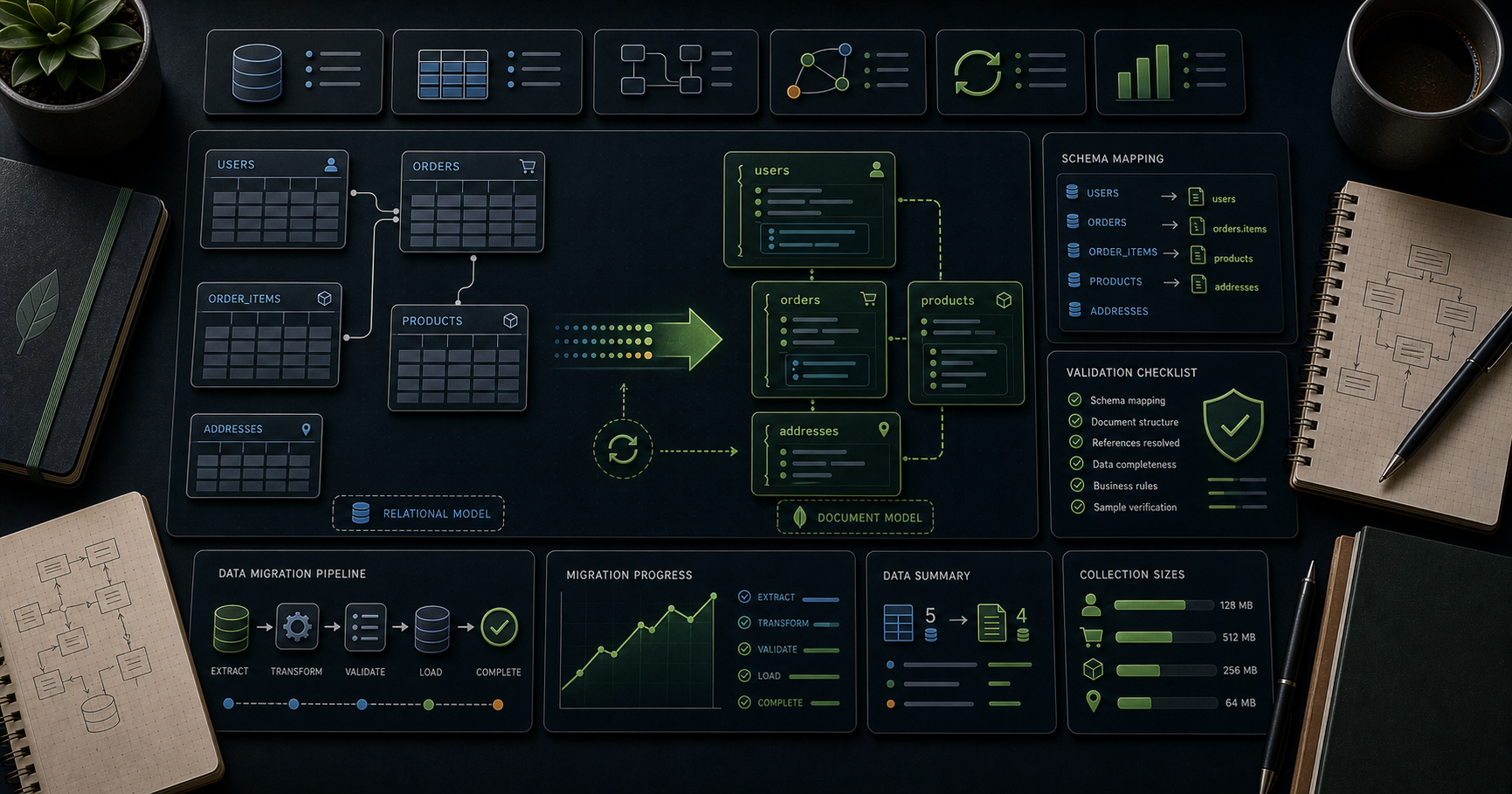
MongoDB Course — 23 · Migrating from SQL / Postgres to MongoDB
You have a Postgres / MySQL / Oracle workload. You want to move it to MongoDB — perhaps because the access pattern is document-shaped, the schema is changing too fast for migrations, or scaling write throughput requires sharding. The migration is half schema redesign, half data movement, half cut-over choreography. This post is the playbook: schema-mapping principles, data-load tooling (mongoimport, AWS DMS, Striim, custom ETL), dual-write strategies, staged cut-over, rollback plan, and the common traps.
> Series map: 20 Outbox → 21 CQRS+ES → 22 RAG → 23 SQL→Mongo migration (this post) → 24 Kafka + Debezium → … → 29 K8s + mongosync + cost.
Learning Outcome
- Decide whether the workload should move at all (and which parts).- Map relational schema to document model using Post 07's patterns.- Choose a data-movement strategy (full reload, dual-write, change-data-capture).- Implement the staged cut-over with rollback gates.- Avoid the 6 most common migration disasters.
Chapter 1 — Should you migrate?
Honest answer first: most SQL workloads should stay on SQL. Migration is expensive + risky. Strong reasons to move:
- Schema flexibility required (per-tenant custom fields, fast product iteration, polymorphic items).- Write throughput beyond what Postgres can vertical-scale.- Hierarchical / document-shaped data (forms, content, configs, complex products) that's painful to join.- Horizontal scaling + multi-region + sharding required.- Operational simplicity at low ops headcount (Atlas managed > self-hosted Postgres cluster).
Weak reasons:
- "NoSQL is modern."- "We want to avoid joins" (you'll write joins as either way).- "We need higher performance" (often a Postgres index would have fixed it).
Often the right answer is migrate a subset — the parts where the document model genuinely fits — and keep the rest in Postgres. The two coexist via outbox / CDC / app-side composition.
Chapter 2 — Schema mapping principles
Re-read Post 07 (Schema Design). Then map:
| SQL pattern | MongoDB pattern ||-------------|------------------|| 1:1 child table | embed sub-document || 1:few (≤ 100) child rows | embed array || 1:many (unbounded) child rows | separate collection + ref || many:many through join table | references both ways (+ counts denormalised) || polymorphic via STI (single table inheritance) | polymorphic pattern (Post 07 Ch 4) — discriminator field || polymorphic via CTI (class table inheritance) | one collection with discriminator || tree (adjacency list) | parent ref or ancestor array (Post 07 Ch 9) || audit history table | separate immutable history collection or Event Sourcing (Post 21) || timestamps columns | embedded or top-level Date fields || JSON column in Postgres | top-level fields directly || sequence / SERIAL primary key | ObjectId (Mongo default) or keep numeric per use || view | materialised view via (Post 06) || trigger | change stream (Post 12) or Atlas Trigger (Post 16) |
Worked mapping — e-commerce orders
Postgres:
MongoDB:
The trade-off: the join you ran 1,000× per second goes away; product name changes don't retroactively rewrite past orders (which is usually correct anyway). A handful of cross-order reports use now and run nightly via .
Chapter 3 — Data movement strategies
Pick by downtime tolerance + data size + complexity tolerance.
Strategy A — Full reload (hours of downtime)
1. Freeze writes to source.2. Extract source → transform → load into Mongo.3. Cut DNS / connection string over.4. Resume writes against Mongo.
OK for: < 100 GB and you can take a maintenance window.
Strategy B — Dual-write at app layer (low downtime)
1. App writes to both Postgres + Mongo for new operations.2. Backfill historical data via ETL.3. Read-shadow: in parallel with reads from Postgres, fetch from Mongo + log differences.4. Switch reads to Mongo when shadow shows parity.5. Stop writes to Postgres.
OK for: medium-size apps where you control the write path.
Strategy C — CDC-driven (best for large, can't-downtime)
1. Tail Postgres WAL via Debezium (or AWS DMS, Striim, Estuary, Airbyte).2. Transform + write to Mongo continuously.3. After sync catches up + remains in sync for a while, cut reads over.4. After cut-over, drain Postgres writes; flip back-flow off.
OK for: large databases, strict uptime requirements, polyglot teams.
Strategy D — Strangler fig
- New features write to Mongo only.- Old features stay on Postgres.- Migrate one feature at a time over months.
OK for: legacy systems where a big-bang move is too risky.
Chapter 4 — Tooling
mongoimport
CSV / TSV / JSONL → MongoDB.
For one-shot loads of dumps.
mongosh load
Run JS scripts against the cluster:
Useful for transforming on insert.
AWS DMS (Database Migration Service)
Continuously replicates Postgres / MySQL / Oracle / SQL Server → MongoDB Atlas. Configurable transformations (rename columns, denormalise child rows into arrays via "JSON-encoded selectors").
Pros: managed; one of the easiest CDC paths to Atlas. Cons: AWS-only; transformations limited.
Debezium + Kafka + Mongo Kafka Sink Connector
Debezium reads Postgres WAL → Kafka → MongoDB Kafka Connector applies events to Atlas. Most flexible (any transformations via Kafka Streams). More moving parts.
Post 24 covers this stack.
Custom ETL
For non-trivial denormalisation (joining 5 tables into one document), write a script:
Use for throughput; chunk to memory-safe batches; checkpoint progress so resumes are cheap.
Striim, Airbyte, Estuary, Hevo, Fivetran
Managed ETL platforms that handle Postgres → Mongo with UI-driven transformations + monitoring. Cost money; save weeks.
Chapter 5 — Dual-write strategy walk-through
Properties:
- Postgres is still source of truth — Mongo failures don't break the user request.- Mongo writes are idempotent (linked by ) — re-runnable.- Backfill script picks up rows in Postgres not yet in Mongo.
Read-shadow phase
Run for days/weeks until diffs are rare + understood. Then flip reads to Mongo for some endpoints; eventually all.
Chapter 6 — Staged cut-over (CDC strategy)
Gates between steps: error budget; latency budget; data-parity assertions. Don't proceed without crossing them.
Rollback plan at each gate:
- T3-T4: trivial — route reads back to Postgres.- T5: still possible — Postgres data is fresh until T6.- T6+: harder — need reverse CDC or accept the cut.
Chapter 7 — Validation
After load (or continuously during CDC):
Automate. Run in CI. Alert on regressions.
For large collections use statistical sampling + checksums per shard / per day rather than full equality.
Chapter 8 — Application-layer changes
The migration isn't just data movement — your code changes too.
| SQL idiom | MongoDB equivalent ||-----------|---------------------|| | embed first; only when must || | + or 2-step query || + window functions | + || + + | sort + skip (small) or range pagination (big) || Transactions across many tables | rethink with single-doc atomicity + embedded data first || Stored procedures | service-layer code || Triggers | change streams || Views | aggregation pipelines + materialised views || | text index, regex (left-anchored), Atlas Search || ORMs | Mongoose / Beanie / Prisma / official driver |
Plan the code refactor in parallel with the data move. Don't try to make Mongo behave like Postgres — you'll get worst of both.
Chapter 9 — Common pitfalls
| Pitfall | Cause | Fix ||---------|-------|-----|| Lift-and-shift schema | one Mongo collection per SQL table | redesign for document shape || 50 s per request | over-normalised | denormalise / embed || ObjectId vs numeric ID mismatch | app expects integer | keep numeric IDs during transition || Date type conversion fails | timezone / format inconsistencies | normalise to ISO 8601 UTC || Foreign-key constraints lost silently | Mongo doesn't enforce | app-layer validation + tests || Sequence ID gaps | new ObjectIds vs SERIAL | use new sequence or rely on ObjectId ordering || Migration script OOM on big tables | not batching | chunk + checkpoint || Forgot indexes on Mongo | full collection scans in prod | create indexes BEFORE traffic || CDC lag during big writes | undersized destination | scale Atlas tier before cut-over || No rollback plan | got stuck after T6 | dual-write until you're 100% sure || Bigger bill than expected | wrong tier sizing | benchmark + size with safety margin |
Chapter 10 — Rollback patterns
If Mongo turns out wrong (worse perf, missing feature, business decision change):
- During dual-write window: trivial. Switch back, drop Mongo data.- After cut-over but Mongo still has CDC back to Postgres: route reads back to Postgres, stop write CDC, keep Mongo as warm standby until decision.- After full cut: you need a reverse migration. Same playbook, opposite direction. Cost as much as the original.
Plan rollback explicitly before T0. Document the decision points.
Practice Exercises
Exercise 1 — Schema mapping
Take a Postgres schema you know (e.g., from a previous project). Map to Mongo collections following Post 07. Note which tables embed and which stay as references.
Exercise 2 — mongoimport
Export one table to CSV from Postgres. into Mongo. Verify counts + spot-check.
Exercise 3 — Dual-write
Implement Chapter 5's dual-write. Insert 1000 orders; confirm both DBs have them. Kill Mongo connectivity mid-test; confirm Postgres still works + Mongo is backfillable.
Exercise 4 — Read-shadow
Implement the shadow comparator. Run 1000 reads; surface diffs. Fix any.
Exercise 5 — CDC PoC
Set up Debezium reading from a local Postgres into Kafka. Configure a Mongo sink. Insert into Postgres; see in Mongo within seconds. (Detailed walkthrough in Post 24.)
Exercise 6 — Staged cut-over plan
For a hypothetical 500 GB Postgres workload, write the full cut-over runbook with T0…T7 + rollback at each step.
Cheat-sheet
| What | How ||------|-----|| First | should you migrate at all? || Map schema | follow Post 07 patterns || Strategy | A (full) / B (dual-write) / C (CDC) / D (strangler) || Tools | mongoimport / DMS / Debezium / Airbyte / custom ETL || Dual-write | source-of-truth source; mirror to Mongo idempotent || Read-shadow | parallel read; log diff; build trust || CDC | Debezium WAL → Kafka → Mongo Sink || Cut-over | gradual % shift on reads; gated by error/latency budget || Validation | counts + sampled equality + aggregate sums || Indexes | create before traffic || Rollback | dual-write window keeps it cheap || Code changes | as much work as data move || Strangler fig | for legacy systems |
What's next
Post 24 covers Kafka + Debezium MongoDB CDC — how to plug MongoDB into Kafka topics in both directions (source + sink) and the patterns that power the migrations + CQRS architectures.
References
- AWS Database Migration Service to MongoDB- Debezium Postgres connector- MongoDB Kafka Connector- Airbyte Postgres → MongoDB- NoSQL Distilled by Pramod Sadalage + Martin Fowler — classic schema-modeling perspective.
> Note: this post is in progress. Planned additions: full DMS task config example; reverse-migration playbook; multi-region migration considerations.
MongoDB Course — 22 · Production RAG Build — Atlas Vector + LangChain + OpenAI
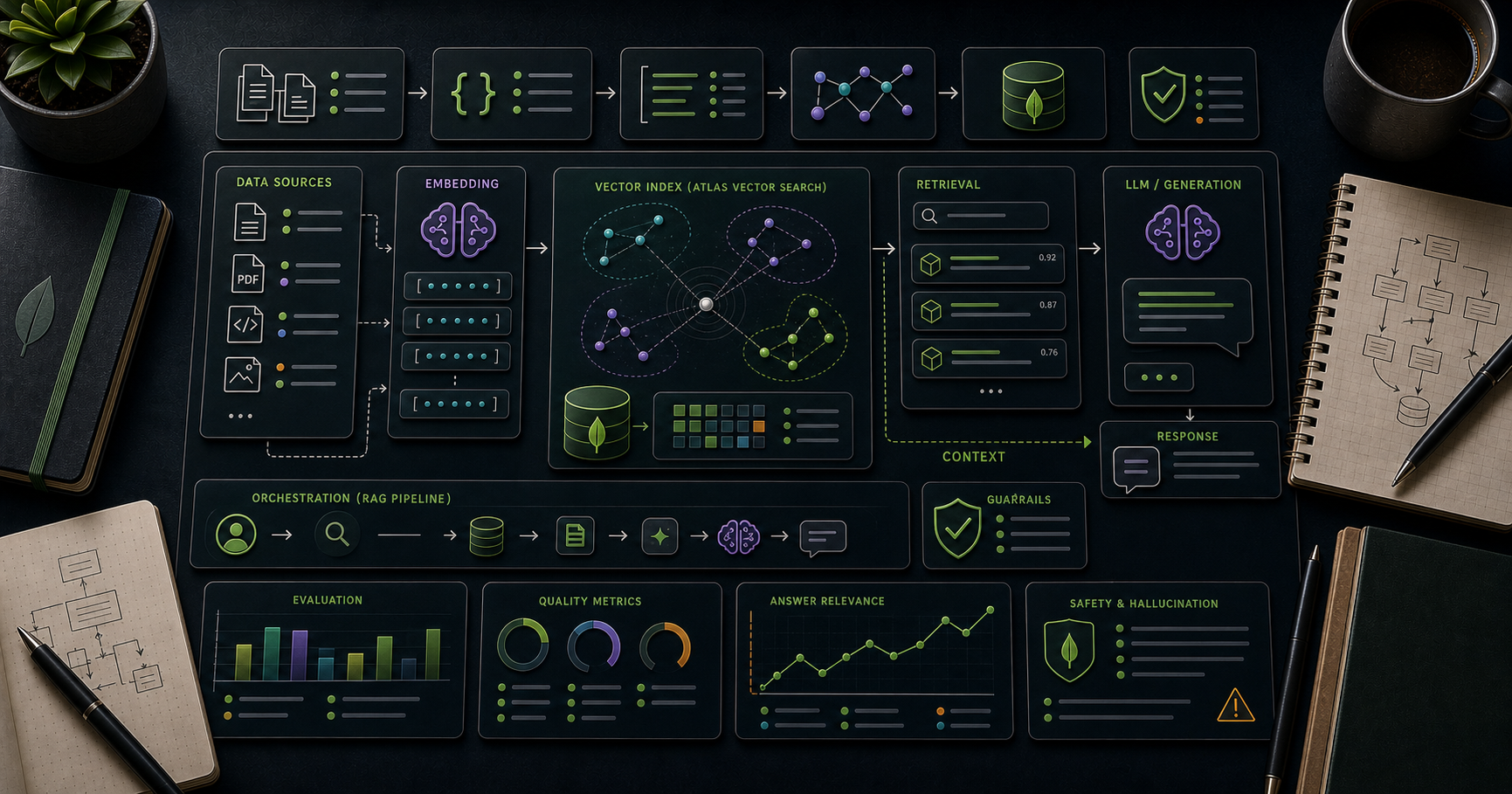
Post 16 introduced Atlas Vector Search. This post builds an end-to-end production-shaped RAG (Retrieval-Augmented Generation) app on top of it: chunking + embedding the corpus, indexing into Atlas, querying with hybrid (lexical + semantic) retrieval, optional reranking, prompt assembly, streaming the LLM response, observability + cost tracking, and the production guardrails (rate limits, citation, evaluation). The framework is LangChain (Python); the embedder is OpenAI text-embedding-3-large; the LLM is GPT-4o (any equivalent works).
> Series map: 19 Beanie+FastAPI → 20 Outbox → 21 CQRS + ES → 22 RAG Production Build (this post) → 23 SQL→Mongo migration → … → 29 K8s + mongosync + cost.
Learning Outcome
- Chunk + embed + index a document corpus into Atlas Vector Search.- Retrieve with vector + lexical + filter (hybrid).- Rerank with a cross-encoder when needed.- Assemble prompts with citations.- Stream the LLM response back to clients.- Track cost + latency + relevance per query.- Evaluate retrieval quality with a small offline eval set.
Chapter 1 — Why MongoDB for RAG
The naïve RAG stack is:
Mongo + Atlas Vector Search replaces a separate vector DB:
- Documents + their embeddings + their metadata live in one collection in one database.- Hybrid search (lexical + vector) is one pipeline (Post 16 Ch 2).- Filter on metadata (tenant, recency, category) alongside vector search.- Same backup / monitoring / connection-pool patterns as the rest of your Mongo workload.- No data sync between document store + vector store.
Trade-off vs Pinecone / Weaviate / pgvector: Atlas Vector Search is HNSW only (no IVF or hybrid index types in 2026); cluster cost scales with index size. For < a few hundred million vectors, Atlas wins on operational simplicity.
Chapter 2 — Ingest pipeline — chunk + embed + insert
Chunking guidelines:
- 800-1200 tokens per chunk for general documents. Smaller for FAQs (200-400); larger for narrative text (1500-2000).- Overlap of 10-15 % to preserve context across boundaries.- For code / structured docs, split at structural boundaries (functions, sections).
Embedding batch size: OpenAI accepts up to 2048 inputs per call; tune to your rate limit. Batch dramatically reduces cost + latency.
Index the embedding (Atlas UI or API)
Also create an Atlas Search lexical index on for hybrid (Chapter 4).
Chapter 3 — Retrieval — vector
Knobs:
- : HNSW search width. Higher = better recall + slower. Start 200; raise to 500-1000 if recall is bad.- : top-k to return.- : pre-filters narrow the search space. Big wins for multi-tenant or category-scoped queries.
Chapter 4 — Hybrid retrieval (lexical + vector)
Vector search misses exact-keyword hits; lexical misses semantic paraphrases. Combine for best recall.
The weights (0.6 / 0.4) are workload-dependent — tune with an eval set (Chapter 8).
A better scoring approach is Reciprocal Rank Fusion (RRF) — combine ranks, not raw scores:
Atlas + the LangChain integration provide hybrid retriever helpers that do this for you.
Chapter 5 — Optional reranking
Hybrid retrieval typically returns 20-50 candidates. A cross-encoder reranker scores each candidate against the query more accurately (slow per pair, fast on small batches).
When to add reranking:
- Quality matters more than 50-100 ms latency.- You're already calling Cohere / OpenAI / Jina for embeddings.- Hybrid alone isn't returning the right doc top-1.
Skip when latency matters more than relevance lift.
Chapter 6 — Prompt assembly with citations
Key rules baked into the prompt:
- Use only context.- Cite numerically (cheap to render in UI).- Refuse when context is insufficient (mitigates hallucination).
The UI then maps to the actual URLs from .
Chapter 7 — LLM call + streaming
In FastAPI:
Stream as Server-Sent Events (SSE) for a chatty UI feel.
Chapter 8 — Evaluation
A small eval set is the difference between "I think it's good" and "I know it's improving".
Build 50-200 queries with the expected source(s). Run retrieval; measure:
- Recall@k — was the right doc in the top-k?- MRR — mean reciprocal rank of the first correct doc.- End-to-end accuracy — manually + via LLM-judge on a sample.
Run on every PR that touches retrieval. CI gate on regression > X %.
LangChain ships an module; LangSmith provides hosted eval + traces; ragas is a popular OSS framework for RAG-specific metrics.
Chapter 9 — Observability + cost
Track per request:
- Query string + tenant + filters.- Embedding tokens (input length).- Retrieved chunk IDs + scores (for offline replay).- Reranker latency.- LLM input + output tokens.- End-to-end latency.
Persist to a collection or use LangSmith / Helicone / Langfuse. Use this data to:
- Identify slow queries.- Estimate per-query cost (embedding tokens × embedding price + LLM tokens × LLM price).- Find queries with low retrieval quality (no high-score matches).
Atlas Charts on the collection gives quick dashboards.
Chapter 10 — Production guardrails
| Guardrail | Why ||-----------|-----|| Rate limit per user / tenant | LLM calls are slow + expensive || Max input length validation | refuses crafted huge inputs || PII / secret scrubbing in inputs + outputs | privacy + compliance || Citation enforcement | hallucination mitigation; user trust || Refusal on low-confidence retrieval | "I don't have the information" beats wrong answers || Logging with masking | debug without leaking || Eval-gated deploys | CI on RAG quality || A/B test retrieval strategies | data-driven tuning || Cost alerts per tenant | catch runaway usage || Streaming | better UX, lower perceived latency || Cache identical question answers per tenant (with TTL) | cost saver |
Chapter 11 — Common pitfalls
| Pitfall | Cause | Fix ||---------|-------|-----|| Embeddings dimension mismatch | swapped model didn't rebuild index | rebuild index when changing embedder || Low recall with high | too small | raise to 500-1000 || Mixed tenants in results | no filter on metadata | add to || LLM ignores context, hallucinates | weak system prompt | strengthen "USE ONLY context"; refusal instruction; eval || Latency spikes | reranker on every query | rerank top-20 only; or skip when not needed || Cost spike | one user spamming | rate-limit + cache identical Qs || Stale answers after document update | embeddings not updated | change-stream-driven re-embed (Post 12) || Long context blowing token limit | too many chunks in prompt | smaller ; smaller chunks || Reranker different lang than docs | language mismatch | use multilingual rerank model || Eval set drift | new feature areas not covered | grow eval set quarterly |
Practice Exercises
Exercise 1 — Ingest a small corpus
Download 50 markdown docs (your repo's docs / Wikipedia subset). Chunk + embed + insert. Build the vector index.
Exercise 2 — Vector-only retrieval
Endpoint that takes a query, runs , returns top-5 chunks + scores. Test 10 questions; rate manually.
Exercise 3 — Hybrid retrieval
Add lexical ( text) to the pipeline. Compare top-5 across vector / lexical / hybrid for the same 10 questions.
Exercise 4 — Reranker
Add Cohere rerank step after hybrid. Confirm top-1 quality improves on questions where exact keywords matter.
Exercise 5 — Streaming endpoint
Wire the streaming pipeline into FastAPI SSE. Render in a small HTML page that progressively displays tokens.
Exercise 6 — Eval harness
Build a 20-question eval set with known gold chunks. Run . Tune , chunk size, reranker on/off; track which combination wins.
Cheat-sheet
| What | How ||------|-----|| Embedder | OpenAI (3072 dim) or (1536) || LLM | GPT-4o / Claude / Gemini — interchangeable || Chunk size | 800-1200 tokens, 10-15 % overlap || Index | Atlas Vector Search HNSW + filter fields || Pre-filter | metadata.tenant / category / date inside || Hybrid | + lexical + RRF combination || Rerank | cross-encoder (Cohere, Jina, etc.) on top-20 || Prompt | system="use only context"; cite with [n] || Stream | SSE / chunked HTTP || Eval | Recall@k / MRR / end-to-end accuracy || Trace | persist per request → collection || Cost | track input + output tokens; rate-limit; cache || Guardrails | refusal on low-confidence; citations; PII scrub || Re-embed on doc change | change stream → re-embed → upsert chunks |
What's next
Post 23 covers migrating from SQL / Postgres to MongoDB — schema-mapping principles, data-load tooling (mongoimport, AWS DMS, custom ETL), dual-write strategies, and the staged cut-over playbook.
References
- Atlas Vector Search docs- LangChain MongoDB integration- LlamaIndex MongoDB integration- LangChain × MongoDB partnership announcement- ragas — RAG evaluation framework- Anthropic + OpenAI prompt engineering guides — system prompt patterns.
> Note: this post is in progress. Planned additions: full chat UI in Next.js; GraphRAG with ; agentic loop (tool-use) example; cost dashboards.
MongoDB Course — 21 · CQRS + Event Sourcing on MongoDB
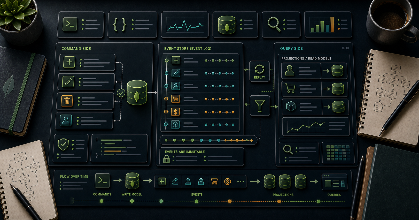
CQRS (Command Query Responsibility Segregation) separates write models from read models. Event Sourcing treats the immutable event log as the source of truth — current state is a projection of replayed events. Both are architectural patterns, not Mongo features — but MongoDB fits them especially well: change streams as the projection bus (Post 12), for materialised views (Post 06), aggregation for replaying events, transactions for atomic event-store appends (Post 09). This post covers when each pays off, the canonical models, the trade-offs vs CRUD, and a worked order-management example end-to-end.
> Series map: 19 Beanie+FastAPI → 20 Outbox → 21 CQRS + Event Sourcing (this post) → 22 RAG → ... → 29 K8s + mongosync + cost.
Learning Outcome
- Define CQRS and recognise when it earns its complexity.- Define Event Sourcing and the event-store schema in MongoDB.- Project events into read models via change streams.- Replay history for new projections + bug fixes.- Handle snapshots + projection rebuilds.- Combine outbox + CQRS + ES into a clean architecture.
Chapter 1 — CQRS in one paragraph
A normal CRUD app uses one model for reads and writes — same schema, same indexes, same database. CQRS splits them: command side handles writes (often normalised, validated, transactional), query side holds one or more read models optimised per use case (denormalised, fast). The read models are updated by events the command side publishes — usually asynchronously.
Benefit:
- Read models match exactly the queries they serve → simple + fast.- Read + write scale independently.- Multiple read models per command model (one for search, one for analytics, one for a mobile API).
Cost:
- More moving parts.- Read-after-write delay (eventual consistency).- Operational complexity.
Use CQRS when one of: read volume >> write volume; queries diverge wildly from write shape; you already need an outbox + projections.
Chapter 2 — Event Sourcing in one paragraph
Instead of storing current state, store every change as an immutable event. Current state is computed by replaying events. Events are append-only — the most reliable storage primitive in databases.
Benefits:
- Full audit trail for free.- New projections retroactively built from history.- Bug fixes can replay events through corrected code.- Time-travel debugging.
Costs:
- Reads must aggregate events (use snapshots + projections).- Schema evolution of events is forever — versioning matters.- Higher mental + ops load than CRUD.
Use ES when one of: regulatory audit trail mandatory; the domain is genuinely event-shaped (orders, payments, IoT, ledger systems); you need to replay history for new analytics or bug correction.
ES + CQRS combine naturally — ES is the command-side event log, CQRS is the read-side projections.
Chapter 3 — When NOT to use CQRS / ES
- A CRUD app with simple reads + writes — KISS.- Small team / small product — overhead > benefit.- Tight read-after-write requirements with no tolerance for eventual consistency.- "Because it sounds modern" — biggest reason teams regret it.
Default = CRUD. Add CQRS only when reads + writes genuinely diverge. Add ES only when the audit-or-replay property is mandatory.
Chapter 4 — Event-store schema
Constraints:
- unique — prevents concurrent appends with the same version. Acts as optimistic concurrency control.- Append-only — never update or delete events.
Use TTL only on very long-term retention if regulation allows. Most ES systems keep events forever (or in cold storage after N years).
Chapter 5 — Command handlers (write side)
A command handler:
1. Loads the aggregate by replaying its events.2. Validates the command against current state.3. Generates new events.4. Appends them with the next sequential .
Concurrency: two handlers trying to append for the same aggregate → one wins, the other gets . The losing handler retries by re-loading the aggregate (now at version N+1) + reapplying validation.
Chapter 6 — Projections (read side)
A projection is a read model derived from events. One projection per query pattern.
Projection: current order view
A projection process change-streams (Post 12) and updates the view:
The read endpoint:
Read side never touches the event log directly. Fast. Indexed. Schema designed for the read pattern.
Multiple projections
Add a keyed by , an view, a Atlas Search index — each is a different consumer of the event stream.
To add a new view: write the projection code, replay events from the beginning (no resume token), let it catch up, switch reads over.
Chapter 7 — Snapshots
Replaying thousands of events per command load is slow. Periodically write a snapshot of the aggregate state, then load .
Take snapshots every N events (e.g., every 50) or on a schedule. Command handler loads snapshot + events with .
Snapshots are derived data — disposable. Wipe + rebuild from events if your apply logic changes.
Chapter 8 — Rebuilding projections
Bug in projection code? Wrote bad state? Rebuild from scratch:
Or use + sort by (events sorted naturally by ObjectId time) instead of change stream for a one-shot rebuild.
This retroactive correctness is one of the headline benefits of ES — no other persistence model lets you "just rerun history with the new code".
Chapter 9 — Event versioning
Events live forever. Their schema must evolve gracefully.
Patterns:
1. Add a field per event type + handle each version in the projection.2. Upcast old events to the new shape at read time.3. Migration events — emit a new event ("schema migrated to v2") rather than mutating history.
Never mutate old events. The event log is sacred — modifying it breaks every projection's correctness.
Chapter 10 — Worked end-to-end architecture
Three deployables:
1. Command service — accepts commands, validates against loaded aggregate, appends events.2. Query service — reads from projection collections.3. Projection workers — one or many, each tail change stream + update one view.
Optional: outbox alongside events for publishing to Kafka (Post 20) — events going to external systems.
Chapter 11 — Trade-offs vs CRUD
| | CRUD | CQRS | CQRS + ES ||---|------|------|-----------|| Code complexity | low | medium | high || Read speed | depends on index | optimal (purpose-built views) | optimal || Write speed | direct mutation | direct mutation | append-only (very fast) || Audit trail | manual | manual | free || Replay history | impossible | impossible | core feature || Read-after-write | strong (single DB) | eventual (projection lag) | eventual || Schema evolution | migrations | migrations | event versioning || Best for | most apps | read-heavy / divergent | regulated / event-shaped |
The simplest pattern that meets your requirements wins. CQRS adds complexity; only pay for it when it earns its keep.
Chapter 12 — Common pitfalls
| Pitfall | Cause | Fix ||---------|-------|-----|| Eventual consistency surprises in UI | read immediately after write | optimistic UI; or read-from-command-side fallback for the actor's own writes || Projection stuck on a bug | one bad event halts the worker | log + skip the bad one + alert; never panic-mutate the event log || Aggregate load slow | thousands of events | snapshots every N events || Lost data on schema migration | upcasting bug or missed event version | exhaustive tests on every event type version || Sharded cross-shard transaction | aggregate scattered across shards | shard key starts with || Projection worker DLQ overflowing | downstream issue | back-pressure; alert; never silently drop || Wrong projection idempotency | duplicates inflate counts | dedupe by event || ES adopted on a CRUD-friendly domain | overengineering | rollback to CRUD; lessons learned |
Practice Exercises
Exercise 1 — Event store
Build the collection from Chapter 4 with the unique index. Append 3 events for one aggregate. Try to append a duplicate — confirm it fails.
Exercise 2 — Command handler
Implement and . Load the aggregate, validate, emit the event. Confirm a against an already-paid order is rejected.
Exercise 3 — Projection
Build the projection (Chapter 6). Start the projection worker; run a few commands; confirm the view stays in sync.
Exercise 4 — Snapshot
After 100 simulated events for one aggregate, write a snapshot. Time the load-aggregate function before + after snapshot — confirm speedup.
Exercise 5 — Rebuild
Drop . Replay from the start (single-pass aggregate). Confirm final state matches what was there before.
Exercise 6 — Schema versioning
Introduce a v2 of that renames → . Update the apply function to handle both versions. Replay history; confirm same final state.
Cheat-sheet
| What | How ||------|-----|| CQRS | separate write + read models || ES | events as source of truth || Event store | append-only collection, unique || Concurrency | unique index acts as optimistic CC || Command handler | load → validate → emit event || Projection | change-stream-driven update of a read view || Multiple views | one worker per view per query pattern || Snapshot | periodic state cache; load || Rebuild projection | drop view + replay from start || Event versioning | never mutate; handle each version in apply || Outbox + ES | combine for cross-service publication || When CRUD | most apps; stick with it || When CQRS | reads heavy and divergent || When ES | regulated audit + replay are mandatory || Pitfall | over-engineering when CRUD suffices |
What's next
Post 22 builds a production RAG (Retrieval-Augmented Generation) application end-to-end using Atlas Vector Search + LangChain + an embedder + an LLM.
References
- Designing Data-Intensive Applications — Ch 11.- Implementing Domain-Driven Design (Vaughn Vernon) — events + aggregates.- microservices.io — CQRS- Event Sourcing on the Microsoft Architecture site- Greg Young's writings on ES
> Note: this post is in progress. Planned additions: complete TypeScript sample app; comparison with EventStore DB; saga orchestrator example; aggregate boundary heuristics.
MongoDB Course — 20 · Outbox Pattern + Transactional Event Publishing
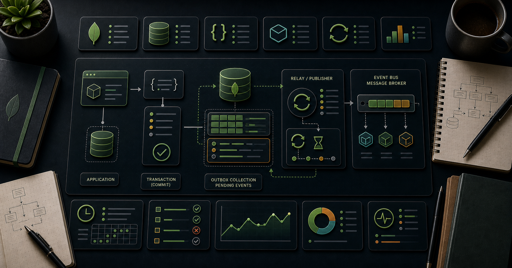
You write to the database. You also need to publish an event ("order placed → send confirmation email"). If those two steps aren't atomic, you'll either lose events (DB committed, queue publish failed) or send duplicates (publish succeeded, DB rolled back). The outbox pattern solves this by treating the event as part of the same DB transaction, then publishing from the outbox to your message bus asynchronously. With MongoDB change streams (Post 12), the publisher is one process tailing the outbox collection — no Kafka Connect, no extra infrastructure. This post covers the full pattern, retry + idempotency + ordering, and the deduplication strategies downstream consumers need.
> Series map: 18 Mongoose → 19 Beanie+FastAPI → 20 Outbox (this post) → 21 CQRS + ES → 22 RAG → ... → 29 K8s + mongosync + cost.
Learning Outcome
- Recognise the dual-write problem.- Build an outbox collection alongside business writes inside one transaction.- Build a change-stream-driven publisher with resume tokens.- Handle at-least-once delivery + downstream idempotency.- Pick between outbox + change streams vs Debezium / Kafka Connect.
Chapter 1 — The dual-write problem
Two failure modes:
- DB insert succeeds, Kafka publish fails → lost event.- Kafka publish succeeds, DB insert fails → phantom event (consumers act on data that doesn't exist).
Neither is acceptable for systems that need consistency between their database state + downstream consumers.
Naive fixes that don't work
- Try-catch + retry: same race, just longer odds.- 2-phase commit across MongoDB + Kafka: not supported across systems.- Eventual consistency + reconciliation: complex; high latency.
The outbox
Write the event as a row in the same database, same transaction as the business mutation. A separate process publishes from the outbox to Kafka / RabbitMQ / SQS / SNS, marking each event as published (or deleting it).
Because the business write + outbox write are in one transaction, they're atomic. The publisher is async + retryable; downstream consumers handle duplicates idempotently.
Chapter 2 — Outbox schema
means unprocessed. The publisher claims, processes, marks.
Chapter 3 — Producer side — transactional write
Both writes commit together or neither does. The business state and the to-be-published event are forever consistent.
Chapter 4 — Publisher — change-stream-driven (the cheap option)
Properties:
- At-least-once delivery — on crash before token persist, we replay.- Resume token persisted after successful publish + mark.- Network blip → retried with backoff, attempts incremented.
This pattern needs no external infrastructure beyond your existing MongoDB. The publisher can run anywhere — a sidecar, a long-running container, a dedicated tiny pod.
Chapter 5 — Publisher — polling fallback
If change streams aren't available (standalone Mongo, very old versions, or a multi-region setup with restricted secondary access):
Higher latency (poll interval) + more DB queries; rock-solid. Use change streams when available, polling as fallback.
Chapter 6 — At-least-once → consumer must be idempotent
Once a publisher delivers at-least-once, consumers will eventually see duplicates (publisher crashed mid-ack, network duplicate, replay after rebuild).
Idempotency patterns:
1. Event ID dedup
Every outbox event has a unique . Consumers track processed IDs (in a "consumedevents" collection, Redis set, etc.). Skip if already processed.
2. Idempotent operations
Make the consumer's side-effect itself idempotent: , upsert by key, "set status to X" rather than increment.
3. Optimistic versioning
Event carries ; consumer rejects updates with .
Combine 1 + 2 for belt-and-braces.
Chapter 7 — Ordering guarantees
Kafka topics + partitions preserve order within a partition. Choose your partition key to match the ordering you need.
For "all events on this order, in order" → key on .For "every event in occurrence order globally" → single-partition topic (low throughput).
Most outbox usage cares about per-aggregate ordering — keying by is the right default.
What if you don't have Kafka?
SQS doesn't preserve order across the queue (unless FIFO with ). SNS doesn't (FIFO topics do). RabbitMQ exchanges + queues do preserve order per queue.
Match destination to the ordering requirement.
Chapter 8 — Backpressure + DLQ
When the downstream is down for hours:
- Outbox grows. Disk usage climbs.- If you have TTL on , you'll lose unpublished events — don't TTL the unpublished portion.- The publisher must implement exponential backoff to avoid hammering a downed downstream.
Dead Letter Queue pattern:
Alert + investigate. Don't silently drop.
Chapter 9 — Outbox + sagas (cross-service workflows)
For workflows spanning services (order → payment → inventory → shipping), combine outbox events with a saga orchestrator. Each step is one service's local transaction + outbox publication. The next service's consumer triggers its step.
If a step fails, the orchestrator publishes a compensating action event → previous services undo.
Outbox makes each step atomic + reliable. The saga adds the cross-step orchestration. Together they're the standard pattern for distributed workflows on document databases.
Chapter 10 — When to use outbox + change streams vs Debezium
| | Outbox + change streams | Debezium MongoDB connector ||---|---|---|| Sync vs async | async publisher process | Kafka Connect cluster || Infrastructure | minimal (just Mongo) | Kafka + Connect || At-least-once | yes | yes || Event format | yours | Debezium envelope (uniform across DBs) || Schema migrations | app-aware | DB-shape only || Best for | one service, simple ops | many services, polyglot DBs into Kafka |
If you already run Kafka + Connect, Debezium is a thin add. If you don't, outbox + change-stream publisher is a cheap, self-contained pattern that scales to many millions of events/day.
Post 24 covers Kafka + Debezium specifically.
Chapter 11 — Common pitfalls
| Pitfall | Cause | Fix ||---------|-------|-----|| Lost events | non-transactional dual-write | use outbox || Phantom events on rollback | publish before commit | publish only from outbox post-commit || Duplicates downstream | at-least-once delivery | idempotent consumers || Publisher process crash → unbounded replay | no resume token persistence | save token after each ack || Outbox bloats | publisher down for long | alert on size; DLQ chronic failures; back-pressure || Wrong partition ordering | random key | partition by aggregateid || Outbox writes blocked by transaction lifetime cap | huge transactions | smaller business transactions || Forgot to mark published | infinite loop re-publishing | always post-ack |
Practice Exercises
Exercise 1 — Build the outbox
Implement from Post 09 that also writes an entry inside the transaction. Confirm both rows appear or neither.
Exercise 2 — Build the publisher
A Node script that change-streams the outbox + prints events to stdout (simulating Kafka). Mark them published.
Exercise 3 — Idempotent consumer
A second script consuming "Kafka" (file or stdin) that dedupes by event against a collection. Replay the same events twice; confirm the side effect runs once.
Exercise 4 — Crash recovery
Kill the publisher mid-batch. Restart. Confirm no event is lost (you may see duplicates — the consumer dedups them).
Exercise 5 — DLQ
Make the consumer fail for a specific eventtype. After 10 attempts, move to . Confirm.
Exercise 6 — Compare to Debezium
(If Kafka available.) Set up Debezium MongoDB source on the same collection. Compare event shape + ordering + ops surface.
Cheat-sheet
| What | How ||------|-----|| Problem | DB write + external publish not atomic || Solution | write event to collection inside same transaction || Publisher | tail outbox via change stream → publish → mark || Persistence | save resume token AFTER successful publish + mark || Delivery | at-least-once || Consumer | idempotent — dedup by event or use idempotent ops || Ordering | partition by in Kafka || Backpressure | back-off; alert on outbox size; DLQ chronic failures || TTL | only on || Alt: Debezium | when Kafka + Connect already in your infra || Sagas | outbox per service + cross-service orchestrator |
What's next
Post 21 covers CQRS + Event Sourcing on MongoDB — separate read + write models, event-stream as source of truth, materialised projections, and the patterns that make them work without overengineering.
References
- Outbox Pattern (microservices.io)- Debezium Outbox Event Router- MongoDB Change Streams- Designing Data-Intensive Applications by Martin Kleppmann — Ch 11 (stream processing).
> Note: this post is in progress. Planned additions: full TypeScript example service with outbox + publisher + idempotent consumer; Kafka topic partitioning rules; outbox + sagas worked example.
Linear Algebra — 03 · Linear Maps, Change of Basis and Determinants
Up to now a matrix has been a table of numbers that you multiply and row-reduce. This post changes the point of view: a matrix is only a description of a linear map, written in one particular pair of bases. Change the bases and the same map gets a different matrix. That idea explains why rank, trace and determinant are "real" properties of a map while individual entries are not, and it is the doorway to eigenvalues in the next post. The second half of the post builds the determinant from three simple rules, proves the key facts (product rule, invertibility test, Cramer's rule), and shows what the number means geometrically: the factor by which a map scales area or volume, with a sign for orientation.
> Series map: 00 Vectors & Linear Systems → 01 Matrix Algebra, Inverses & LU → 02 Vector Spaces, Basis & Dimension → 03 Linear Maps, Change of Basis & Determinants (this post) → 04 Eigenvalues & Diagonalization → 05 Inner Products, Spectral Theorem & SVD.
Learning Outcome
- Decide whether a given function between vector spaces is linear, and find its kernel and image.- State and prove the rank–nullity theorem for linear maps, and use it to relate injective, surjective and invertible.- Write the matrix of a linear map relative to any bases, and explain why composition of maps is the matrix product.- Convert coordinates between bases, and compute the matrix of a map in a new basis with $P^{-1}AP$.- Recognise rotations, reflections, shears, projections and scalings in $\mathbb{R}^2$ from their matrices.- Define the determinant by its three axioms, compute it by cofactor expansion and by elimination, and prove $\det(AB) = \det A \det B$.- Interpret $\lvert\det A\rvert$ as a volume scaling factor and the sign of $\det A$ as orientation.- Solve small systems with Cramer's rule, and explain why it is not used for large ones.
Chapter 1 — Linear maps
Terminology
- Vector space $V$ over $\mathbb{R}$ — as in Linear Algebra 02: a set with addition and scalar multiplication obeying the eight axioms. Everything in this post also works over $\mathbb{C}$ or any field.- Linear map (linear transformation) $T: V \to W$ — a function that respects addition and scalar multiplication (definition below). When $V = W$ it is also called a linear operator on $V$.- Domain $V$ and codomain $W$ — where inputs live and where outputs are allowed to land.- Kernel (null space) $\ker T = \{v \in V : T(v) = 0\}$.- Image (range) $\operatorname{im} T = \{T(v) : v \in V\}$.- Rank of $T$ — $\dim \operatorname{im} T$. Nullity of $T$ — $\dim \ker T$.- Injective (one-to-one) — $T(u) = T(v)$ implies $u = v$. Surjective (onto) — $\operatorname{im} T = W$. Bijective — both.- Isomorphism — a bijective linear map. $V$ and $W$ are isomorphic, written $V \cong W$, if an isomorphism exists.- $Pn$ — polynomials of degree at most $n$ with real coefficients; $\dim Pn = n + 1$.
Definition
A function $T: V \to W$ is linear if for all $u, v \in V$ and all scalars $c$:
$$T(u + v) = T(u) + T(v), \qquad T(cv) = c\,T(v).$$
The two conditions combine into one: $T(c1 v1 + c2 v2) = c1 T(v1) + c2 T(v2)$. By induction, a linear map sends every linear combination to the same combination of the images. Taking $c = 0$ gives $T(0) = 0$: a linear map always sends zero to zero.
Examples:
1. Matrix maps. For an $m \times n$ matrix $A$, the map $TA: \mathbb{R}^n \to \mathbb{R}^m$, $TA(x) = Ax$, is linear because $A(u+v) = Au + Av$ and $A(cv) = cAv$ (Linear Algebra 01).2. Differentiation. $D: P3 \to P2$, $D(p) = p'$. The sum rule and the constant-multiple rule of calculus are exactly the two linearity conditions.3. Integration. $I: C[0,1] \to \mathbb{R}$, $I(f) = \int0^1 f(x)\,dx$, where $C[0,1]$ is the space of continuous functions on $[0,1]$.4. Evaluation. $E: P2 \to \mathbb{R}^2$, $E(p) = (p(0), p(1))$.5. Transpose. $M \mapsto M^T$ from $m \times n$ matrices to $n \times m$ matrices.
Non-examples:
- Translation $T(x) = x + b$ with $b \neq 0$: $T(0) = b \neq 0$, so it is not linear. (It is called affine.)- $T(x, y) = (x + y, xy)$: $T(2 \cdot (1,1)) = (4, 4)$ but $2\,T(1,1) = (4, 2)$.- $T(x) = \lvert x\rvert$ on $\mathbb{R}$: $T(-1) = 1 \neq -T(1)$.
> Trick: To show a map is not linear, one counterexample is enough — and checking $T(0) = 0$ first catches many cases in one line. To show a map is linear, you must check both conditions for arbitrary inputs.
A linear map is fixed by what it does to a basis
Theorem 1. Let $b1, \dots, bn$ be a basis of $V$ and let $w1, \dots, wn$ be any vectors in $W$. There is exactly one linear map $T: V \to W$ with $T(bi) = wi$ for every $i$.
Proof. Every $v \in V$ has unique coordinates: $v = c1 b1 + \dots + cn bn$ (Linear Algebra 02). Define $T(v) = c1 w1 + \dots + cn wn$. This is well defined because the coordinates are unique. It is linear: if $v$ has coordinates $ci$ and $u$ has coordinates $di$, then $u + v$ has coordinates $ci + di$ and $kv$ has coordinates $kci$, and the formula is linear in the coordinates. It sends $bi$ to $wi$. For uniqueness, any linear $S$ with $S(bi) = wi$ satisfies $S(v) = \sum ci S(bi) = \sum ci wi = T(v)$. ∎
This theorem is the reason matrices work at all: to store a linear map you only need to store $n$ vectors, the images of the basis vectors.
Chapter 2 — Kernel, image and rank–nullity
Kernel and image are subspaces
Proposition 2. For linear $T: V \to W$, $\ker T$ is a subspace of $V$ and $\operatorname{im} T$ is a subspace of $W$.
Proof. $T(0) = 0$, so $0$ is in both. If $T(u) = T(v) = 0$ then $T(u + cv) = 0 + c \cdot 0 = 0$, so the kernel is closed under addition and scaling. If $w1 = T(v1)$ and $w2 = T(v2)$ then $w1 + c w2 = T(v1 + c v2)$ is also in the image. ∎
For a matrix map $TA$, the kernel is the null space $N(A)$ and the image is the column space $C(A)$ from Linear Algebra 02.
Proposition 3. $T$ is injective if and only if $\ker T = \{0\}$.
Proof. If $T$ is injective and $T(v) = 0 = T(0)$, then $v = 0$. Conversely, if $\ker T = \{0\}$ and $T(u) = T(v)$, then $T(u - v) = 0$, so $u - v = 0$. ∎
> Watch out: "The only solution of $T(v) = 0$ is $v = 0$" is a statement about one equation, but it controls every equation $T(v) = w$: each one then has at most one solution. This is the map version of "no free variables" from Linear Algebra 00.
Rank–nullity for linear maps
Linear Algebra 02 proved $\operatorname{rank} A + \dim N(A) = n$ for an $m \times n$ matrix by counting pivot and free columns. Here is the version for maps, with a proof that uses no matrices at all.
Theorem 4 (rank–nullity). Let $V$ be finite-dimensional and $T: V \to W$ linear. Then $\operatorname{im} T$ is finite-dimensional and
$$\dim V = \dim \ker T + \dim \operatorname{im} T.$$
Proof. $\ker T$ is a subspace of the finite-dimensional space $V$, so it has a basis $u1, \dots, uk$ (possibly $k = 0$). By the basis-extension theorem of Linear Algebra 02, extend it to a basis $u1, \dots, uk, w1, \dots, wr$ of $V$, so $\dim V = k + r$. We show that $T(w1), \dots, T(wr)$ is a basis of $\operatorname{im} T$; then $\dim \operatorname{im} T = r$ and we are done.
Spanning. Any vector in the image is $T(v)$ for some $v = \sum ai ui + \sum bj wj$. Since $T(ui) = 0$, we get $T(v) = \sum bj T(wj)$.
Independence. Suppose $\sum cj T(wj) = 0$. Then $T\left(\sum cj wj\right) = 0$, so $\sum cj wj \in \ker T$ and can be written as $\sum di ui$. Then $\sum cj wj - \sum di ui = 0$ is a linear relation among the basis vectors of $V$, so every $cj$ (and every $di$) is zero. ∎
Worked example. $T: \mathbb{R}^3 \to \mathbb{R}^2$, $T(x, y, z) = (x + 2y - z,\ 2x + 4y + z)$. Its matrix is
$$A = \begin{pmatrix} 1 & 2 & -1 \\ 2 & 4 & 1 \end{pmatrix}.$$
Solving $T(v) = 0$: adding the two equations gives $3x + 6y = 0$, so $x = -2y$, and then $z = x + 2y = 0$. The kernel is the line spanned by $(-2, 1, 0)$, so the nullity is 1. Rank–nullity forces $\dim \operatorname{im} T = 3 - 1 = 2$, so the image is all of $\mathbb{R}^2$: $T$ is surjective but not injective.
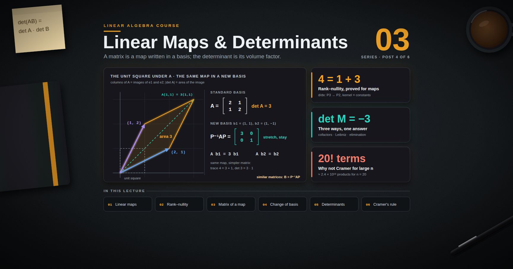
Worked example (no matrix in sight). $D: P3 \to P2$, $D(p) = p'$. The kernel is the constant polynomials (dimension 1). Every $q \in P2$ is the derivative of some cubic, so the image is $P2$ (dimension 3). Check: $4 = 1 + 3$.
Consequences
Corollary 5. Let $T: V \to W$ be linear with $V, W$ finite-dimensional.
1. If $\dim V > \dim W$, then $T$ is not injective (the kernel has dimension at least $\dim V - \dim W > 0$).2. If $\dim V < \dim W$, then $T$ is not surjective (the image has dimension at most $\dim V$).3. If $\dim V = \dim W$, then $T$ injective $\iff$ $T$ surjective $\iff$ $T$ is an isomorphism.
Proof of 3. Injective means $\dim \ker T = 0$, which by rank–nullity means $\dim \operatorname{im} T = \dim V = \dim W$, which means $\operatorname{im} T = W$ (a subspace of full dimension is the whole space). ∎
Part 3 is the abstract form of the invertible matrix theorem from Linear Algebra 01: for a square matrix, "only the trivial solution" and "a solution for every right-hand side" are the same condition.
Theorem 6 (classification by dimension). Two finite-dimensional spaces are isomorphic if and only if they have the same dimension. In particular every $n$-dimensional real space is isomorphic to $\mathbb{R}^n$.
Proof. An isomorphism sends a basis to a basis (it is injective, so independence is kept, and surjective, so the images span), so dimensions agree. Conversely, if $\dim V = n$ with basis $b1, \dots, bn$, the coordinate map $v \mapsto (c1, \dots, cn)$ is linear, injective and surjective. Composing two such maps gives $V \cong \mathbb{R}^n \cong W$. ∎
The inverse of an isomorphism is automatically linear: if $T(u') = u$ and $T(v') = v$, then $T(u' + cv') = u + cv$, so $T^{-1}(u + cv) = T^{-1}(u) + cT^{-1}(v)$.
> Common pitfall: Isomorphic does not mean equal. $P2$ and $\mathbb{R}^3$ are isomorphic, but the isomorphism depends on a choice of basis. There is no single "correct" identification — which is exactly why the next chapter keeps track of bases.
Chapter 3 — The matrix of a linear map
Coordinates
Fix an ordered basis $\mathcal{B} = (b1, \dots, bn)$ of $V$. The coordinate vector of $v$ is the column $[v]{\mathcal{B}} = (c1, \dots, cn)^T$ with $v = \sum ci bi$. The map $v \mapsto [v]{\mathcal{B}}$ is the isomorphism $V \to \mathbb{R}^n$ of Theorem 6. Order matters: swapping $b1$ and $b2$ swaps the first two coordinates.
The matrix relative to two bases
Let $T: V \to W$ be linear, with basis $\mathcal{B} = (b1, \dots, bn)$ of $V$ and $\mathcal{C} = (c1, \dots, cm)$ of $W$. The matrix of $T$ relative to $\mathcal{B}$ and $\mathcal{C}$ is the $m \times n$ matrix
$$[T]{\mathcal{C} \leftarrow \mathcal{B}} = \Big( [T(b1)]{\mathcal{C}} \ \ [T(b2)]{\mathcal{C}} \ \ \cdots \ \ [T(bn)]{\mathcal{C}} \Big).$$
Column $j$ = the $\mathcal{C}$-coordinates of the image of the $j$-th basis vector. With it, applying $T$ becomes matrix multiplication on coordinates:
$$[T(v)]{\mathcal{C}} = [T]{\mathcal{C} \leftarrow \mathcal{B}}\, [v]{\mathcal{B}}.$$
Why: if $v = \sum xj bj$ then $T(v) = \sum xj T(bj)$, and taking $\mathcal{C}$-coordinates (a linear operation) gives $\sum xj [T(bj)]{\mathcal{C}}$, which is the matrix times the column $x$.
The arrow notation $\mathcal{C} \leftarrow \mathcal{B}$ reads right to left: coordinates in $\mathcal{B}$ go in, coordinates in $\mathcal{C}$ come out. When $V = W$ and the same basis is used on both sides, write $[T]{\mathcal{B}}$.
Worked example. $D: P3 \to P2$ with bases $(1, x, x^2, x^3)$ and $(1, x, x^2)$. The images of the basis vectors are $0,\ 1,\ 2x,\ 3x^2$, whose coordinates are the columns:
$$[D] = \begin{pmatrix} 0 & 1 & 0 & 0 \\ 0 & 0 & 2 & 0 \\ 0 & 0 & 0 & 3 \end{pmatrix}.$$
Check with $p = 1 + 2x - x^2 + 4x^3$: $[D]\,(1, 2, -1, 4)^T = (2, -2, 12)^T$, and indeed $p' = 2 - 2x + 12x^2$. The matrix has rank 3 and a one-dimensional null space spanned by $(1,0,0,0)^T$ — the constant polynomial 1 — matching the rank–nullity count above.
Composition is the matrix product
Theorem 7. Let $T: U \to V$ and $S: V \to W$ be linear, with bases $\mathcal{B}, \mathcal{C}, \mathcal{D}$ of $U, V, W$. Then
$$[S \circ T]{\mathcal{D} \leftarrow \mathcal{B}} = [S]{\mathcal{D} \leftarrow \mathcal{C}}\ [T]{\mathcal{C} \leftarrow \mathcal{B}}.$$
Proof. For every $u \in U$: $[S(T(u))]{\mathcal{D}} = [S]\,[T(u)]{\mathcal{C}} = [S]\,[T]\,[u]{\mathcal{B}}$. Taking $u = bj$ (so $[u]{\mathcal{B}}$ is the $j$-th standard column) shows that column $j$ of $[S \circ T]$ equals column $j$ of $[S][T]$. ∎
This is why matrix multiplication is defined the strange row-times-column way: it is the only definition that makes "do $T$, then do $S$" correspond to a product. It also explains why the product is associative (composition of functions is) and generally not commutative (doing things in a different order usually gives a different result). The order is right to left: in $ST$, $T$ acts first.
Two consequences follow at once. $T$ is an isomorphism if and only if its matrix (in any bases) is invertible, and then $[T^{-1}]{\mathcal{B} \leftarrow \mathcal{C}} = \left([T]{\mathcal{C} \leftarrow \mathcal{B}}\right)^{-1}$. And the rank of $T$ equals the rank of any matrix that represents it.
Chapter 4 — Change of basis and similarity
The change-of-basis matrix
Let $\mathcal{E}$ be the standard basis of $\mathbb{R}^n$ and $\mathcal{B} = (b1, \dots, bn)$ another basis. Put the new basis vectors, written in standard coordinates, into the columns of
$$P = P{\mathcal{E} \leftarrow \mathcal{B}} = \big( b1 \ \ b2 \ \ \cdots \ \ bn \big).$$
Then $v = \sum ci bi = P\,[v]{\mathcal{B}}$, that is
$$[v]{\mathcal{E}} = P\,[v]{\mathcal{B}}, \qquad [v]{\mathcal{B}} = P^{-1}[v]{\mathcal{E}}.$$
$P$ is invertible because its columns are a basis. $P$ is simply the matrix of the identity map, $[\mathrm{id}]{\mathcal{E} \leftarrow \mathcal{B}}$: it takes $\mathcal{B}$-coordinates in and gives $\mathcal{E}$-coordinates out.
> Common pitfall: The matrix whose columns are the new basis vectors converts new coordinates to old, not old to new. To get new coordinates you must solve $P c = v$ (or apply $P^{-1}$). Writing the arrow $\mathcal{E} \leftarrow \mathcal{B}$ on every change-of-basis matrix prevents this mistake.
The same map in a new basis
Let $T: \mathbb{R}^n \to \mathbb{R}^n$ have standard matrix $A = [T]{\mathcal{E}}$. Its matrix in the basis $\mathcal{B}$ is found by composing: convert $\mathcal{B}$-coordinates to standard ($P$), apply $T$ ($A$), convert back ($P^{-1}$):
$$[T]{\mathcal{B}} = P^{-1} A P.$$
This is Theorem 7 applied to $T = \mathrm{id} \circ T \circ \mathrm{id}$. For a map between different spaces, with change-of-basis matrices $P$ on the domain and $Q$ on the codomain, the rule is $[T]{\mathcal{C}' \leftarrow \mathcal{B}'} = Q^{-1}\,[T]{\mathcal{C} \leftarrow \mathcal{B}}\,P$.
Worked example. Let $A = \begin{pmatrix} 2 & 1 \\ 1 & 2 \end{pmatrix}$ and take the basis $b1 = (1, 1)$, $b2 = (1, -1)$. Then
$$P = \begin{pmatrix} 1 & 1 \\ 1 & -1 \end{pmatrix}, \quad P^{-1} = \frac{1}{2}\begin{pmatrix} 1 & 1 \\ 1 & -1 \end{pmatrix}, \quad P^{-1}AP = \begin{pmatrix} 3 & 0 \\ 0 & 1 \end{pmatrix}.$$
You can see the diagonal answer directly: $Ab1 = (3, 3) = 3b1$ and $Ab2 = (1, -1) = b2$. In the new basis the map just stretches the $b1$ direction by 3 and leaves the $b2$ direction alone. Now track one vector. $v = (5, 1)$ has $[v]{\mathcal{B}} = P^{-1}v = (3, 2)$, because $3(1,1) + 2(1,-1) = (5, 1)$. In new coordinates the map gives $\operatorname{diag}(3,1)\,(3,2)^T = (9, 2)^T$, and $9(1,1) + 2(1,-1) = (11, 7) = Av$. The two routes agree.
Choosing a basis that makes the matrix diagonal is the whole subject of Linear Algebra 04: $b1$ and $b2$ here are eigenvectors.
Similarity
Square matrices $A$ and $B$ are similar if $B = P^{-1}AP$ for some invertible $P$. Similar matrices are the same linear operator written in two bases. Similarity is an equivalence relation (reflexive with $P = I$, symmetric with $P^{-1}$, transitive with $PQ$).
Anything defined for the operator rather than the table of numbers must be the same for similar matrices. Such quantities are called similarity invariants:
| Invariant | Why it survives $A \mapsto P^{-1}AP$ ||-----------|--------------------------------------|| Rank | rank of the map, which does not depend on coordinates || Trace | $\operatorname{tr}(XY) = \operatorname{tr}(YX)$, so $\operatorname{tr}(P^{-1}(AP)) = \operatorname{tr}((AP)P^{-1})$ || Determinant | product rule (Chapter 6): $\det P^{-1} \det A \det P = \det A$ || Characteristic polynomial, eigenvalues | Linear Algebra 04 |
The trace identity is a one-line calculation: $\operatorname{tr}(XY) = \sumi \sumj x{ij} y{ji} = \sumj \sumi y{ji} x{ij} = \operatorname{tr}(YX)$. Check the example: $\operatorname{tr}A = 4 = 3 + 1$.
> Watch out: Equal invariants do not prove similarity. $I = \begin{pmatrix} 1 & 0 \\ 0 & 1\end{pmatrix}$ and $\begin{pmatrix} 1 & 1 \\ 0 & 1\end{pmatrix}$ have the same rank, trace and determinant, but only $I$ is similar to $I$ (because $P^{-1}IP = I$ for every $P$).
Chapter 5 — Geometry of maps in the plane
The quickest way to read a $2 \times 2$ matrix: its columns are where $e1 = (1,0)$ and $e2 = (0,1)$ land. Draw those two arrows and you have drawn the map, because the unit square goes to the parallelogram they span and every grid line goes to a parallel grid line.
| Map | Matrix | What it does | det ||-----|--------|--------------|-----|| Rotation by $\theta$ | $\begin{pmatrix} \cos\theta & -\sin\theta \\ \sin\theta & \cos\theta \end{pmatrix}$ | turns every vector by angle $\theta$ counter-clockwise | $1$ || Reflection in the line at angle $\theta$ | $\begin{pmatrix} \cos 2\theta & \sin 2\theta \\ \sin 2\theta & -\cos 2\theta \end{pmatrix}$ | mirror image; vectors on the line stay put | $-1$ || Shear | $\begin{pmatrix} 1 & k \\ 0 & 1 \end{pmatrix}$ | slides each point sideways by $k$ times its height | $1$ || Projection onto the line at angle $\theta$ | $\begin{pmatrix} \cos^2\theta & \cos\theta\sin\theta \\ \cos\theta\sin\theta & \sin^2\theta \end{pmatrix}$ | drops each point perpendicularly onto the line | $0$ || Scaling | $\begin{pmatrix} a & 0 \\ 0 & b \end{pmatrix}$ | stretches $x$ by $a$ and $y$ by $b$ | $ab$ |
Where these come from:
- Rotation. $e1$ goes to $(\cos\theta, \sin\theta)$ and $e2$ (at angle $90°$) goes to $(\cos(\theta + 90°), \sin(\theta + 90°)) = (-\sin\theta, \cos\theta)$. For $\theta = 30°$ this gives $\begin{pmatrix} \sqrt{3}/2 & -1/2 \\ 1/2 & \sqrt{3}/2 \end{pmatrix}$.- Projection. With the unit vector $u = (\cos\theta, \sin\theta)$ along the line, the projection of $x$ is $(u \cdot x)\,u = (u u^T) x$, and $uu^T$ is the matrix in the table. It satisfies $P^2 = P$: projecting twice is the same as projecting once.- Reflection. Reflection = $2 \times$ projection $-$ identity (go to the line, then the same distance again). Using $2\cos^2\theta - 1 = \cos 2\theta$ and $2\sin\theta\cos\theta = \sin 2\theta$ gives the table entry. It satisfies $F^2 = I$.
Composition does not commute. Let $R$ be rotation by $90°$ and $F$ reflection in the $x$-axis:
$$R = \begin{pmatrix} 0 & -1 \\ 1 & 0 \end{pmatrix}, \quad F = \begin{pmatrix} 1 & 0 \\ 0 & -1 \end{pmatrix}, \quad FR = \begin{pmatrix} 0 & -1 \\ -1 & 0 \end{pmatrix}, \quad RF = \begin{pmatrix} 0 & 1 \\ 1 & 0 \end{pmatrix}.$$
"Rotate, then reflect" ($FR$) is the reflection in the line $y = -x$; "reflect, then rotate" ($RF$) is the reflection in $y = x$. Two different maps.
A projection is diagonal in the right basis. The projection onto the line $y = 2x$ has standard matrix $\frac{1}{5}\begin{pmatrix} 1 & 2 \\ 2 & 4 \end{pmatrix}$. In the basis $(1, 2), (-2, 1)$ — one vector along the line, one perpendicular to it — its matrix is $\begin{pmatrix} 1 & 0 \\ 0 & 0 \end{pmatrix}$: keep the first coordinate, kill the second. Same map, much clearer matrix.
Chapter 6 — The determinant
Terminology
- Multilinear (in the rows) — linear in each row separately when the other rows are held fixed.- Alternating — the value is $0$ whenever two rows are equal.- Permutation of $\{1, \dots, n\}$ — a bijection $\sigma$ of the set to itself; $Sn$ is the set of all $n!$ of them.- Sign $\operatorname{sgn}(\sigma)$ — $+1$ if $\sigma$ is a product of an even number of swaps, $-1$ if odd. Equivalently $(-1)^{\text{number of inversions}}$, where an inversion is a pair $i < j$ with $\sigma(i) > \sigma(j)$.- Minor $M{ij}$ — the determinant of the $(n-1) \times (n-1)$ matrix left after deleting row $i$ and column $j$. Cofactor $C{ij} = (-1)^{i+j} M{ij}$.
The three axioms
For $2 \times 2$ matrices you know $\det \begin{pmatrix} a & b \\ c & d \end{pmatrix} = ad - bc$. The clean way to generalise is not to guess a formula but to list the properties we want and prove that exactly one function has them.
A function $D$ from $n \times n$ matrices to $\mathbb{R}$ is a determinant function if:
1. (Multilinear) $D$ is linear in each row: $D(\dots, u + cv, \dots) = D(\dots, u, \dots) + c\,D(\dots, v, \dots)$, other rows fixed.2. (Alternating) $D(A) = 0$ if two rows of $A$ are equal.3. (Normalised) $D(I) = 1$.
Theorem 8 (existence and uniqueness). There is exactly one determinant function, written $\det$. Moreover, any function $D$ satisfying axioms 1 and 2 (but not necessarily 3) equals $D(I) \cdot \det$.
Existence is shown by checking that the Leibniz formula below satisfies the three axioms; uniqueness follows because the axioms alone determine the value on every matrix, as the row-operation rules show. A full proof is in Axler (Chapter 9) or Hoffman and Kunze (Chapter 5); here we state it and use it.
What the axioms force: row operations
From the axioms alone:
- Swapping two rows changes the sign. Put $u + v$ in both rows $i$ and $j$. By axiom 2 the value is 0; expanding with axiom 1 gives $D(u,u) + D(u,v) + D(v,u) + D(v,v) = 0$ (other rows omitted), and the first and last terms are 0, so $D(u,v) = -D(v,u)$.- Scaling one row by $c$ multiplies the determinant by $c$ (axiom 1).- Adding a multiple of one row to another leaves the determinant unchanged: $D(\dots, u + cv, \dots, v, \dots) = D(\dots, u, \dots, v, \dots) + c\,D(\dots, v, \dots, v, \dots)$, and the last term is 0.- A zero row gives determinant 0 (scale that row by 0).- A triangular matrix has determinant = product of its diagonal entries. If all diagonal entries are nonzero, row replacements clear the off-diagonal entries without changing $D$, leaving a diagonal matrix, and axiom 1 plus axiom 3 give the product. If a diagonal entry is zero, elimination produces a zero row, so both sides are 0.
These rules are also the fastest way to compute: row-reduce to triangular form, keeping track of swaps and scalings.
Leibniz formula and cofactor expansion
Leibniz formula.
$$\det A = \sum{\sigma \in Sn} \operatorname{sgn}(\sigma)\, a{1\sigma(1)}\, a{2\sigma(2)} \cdots a{n\sigma(n)}.$$
Each term picks one entry from every row and every column. For $n = 2$ there are two terms, $a{11}a{22} - a{12}a{21}$. For $n = 3$ there are six:
$$\det A = a{11}a{22}a{33} + a{12}a{23}a{31} + a{13}a{21}a{32} - a{13}a{22}a{31} - a{11}a{23}a{32} - a{12}a{21}a{33}.$$
Cofactor (Laplace) expansion along row $i$ or column $j$:
$$\det A = \sum{j=1}^{n} a{ij} C{ij} \quad \text{(row } i\text{)}, \qquad \det A = \sum{i=1}^{n} a{ij} C{ij} \quad \text{(column } j\text{)}.$$
The signs $(-1)^{i+j}$ follow a checkerboard starting with $+$ in the top-left corner. Expand along the row or column with the most zeros.
Worked example — three ways. Let
$$M = \begin{pmatrix} 1 & 2 & 3 \\ 4 & 5 & 6 \\ 7 & 8 & 10 \end{pmatrix}.$$
Cofactor expansion along row 1:
$$\det M = 1(5 \cdot 10 - 6 \cdot 8) - 2(4 \cdot 10 - 6 \cdot 7) + 3(4 \cdot 8 - 5 \cdot 7) = 1(2) - 2(-2) + 3(-3) = -3.$$
Leibniz, six terms: $50 + 84 + 96 - 105 - 48 - 80 = 230 - 233 = -3$.
Elimination: $R2 - 4R1$ and $R3 - 7R1$ give rows $(0, -3, -6)$ and $(0, -6, -11)$; then $R3 - 2R2$ gives $(0, 0, 1)$. Only row replacements were used, so the determinant is unchanged: $\det M = 1 \cdot (-3) \cdot 1 = -3$.
> Watch out: The "diagonals" trick (rule of Sarrus) works for $3 \times 3$ matrices only. For $4 \times 4$ it gives 8 terms, but the determinant has $4! = 24$.
The product rule and other properties
Theorem 9. $\det(AB) = \det A \cdot \det B$ for all $n \times n$ matrices $A, B$.
Proof. Fix $B$ and define $D(A) = \det(AB)$. Row $i$ of $AB$ is (row $i$ of $A$) $\times B$, which is linear in row $i$ of $A$, so $D$ is multilinear in the rows of $A$. If $A$ has two equal rows, so does $AB$, so $D(A) = 0$. By the second part of Theorem 8, $D(A) = D(I)\det A = \det(B)\det(A)$. ∎
Theorem 10. $\det A^T = \det A$.
Reason. In the Leibniz formula, the term for $\sigma$ in $\det A^T$ is the term for $\sigma^{-1}$ in $\det A$, and $\operatorname{sgn}(\sigma^{-1}) = \operatorname{sgn}(\sigma)$. As $\sigma$ runs over $Sn$ so does $\sigma^{-1}$. ∎
So every statement about rows also holds for columns: column swaps flip the sign, and so on.
Theorem 11 (the invertibility test). A square matrix $A$ is invertible if and only if $\det A \neq 0$. In that case $\det(A^{-1}) = 1/\det A$.
Proof. Row-reduce: $Ek \cdots E1 A = R$ with $R$ in reduced row echelon form. Each elementary operation multiplies the determinant by a nonzero number ($-1$, $c \neq 0$, or $1$), so $\det A \neq 0 \iff \det R \neq 0$. A square RREF is either $I$ (determinant 1) or has a zero row (determinant 0), and $R = I$ exactly when $A$ is invertible (Linear Algebra 01). For the formula, $\det A \det A^{-1} = \det I = 1$. ∎
Further consequences:
- $\det(cA) = c^n \det A$ for an $n \times n$ matrix (each of the $n$ rows is scaled). For the matrix $M$ above, $\det(2M) = 8 \cdot (-3) = -24$.- Similar matrices have equal determinants, so $\det T$ is well defined for a linear operator $T$: use its matrix in any basis.- For block upper triangular matrices, $\det \begin{pmatrix} A & B \\ 0 & D \end{pmatrix} = \det A \det D$ (with $A$, $D$ square).
> Common pitfall: $\det(A + B) \neq \det A + \det B$ in general. Try $A = B = I2$: the left side is $\det(2I) = 4$, the right side is 2. The determinant is multiplicative, not additive.
Determinant as signed volume
For $n \times n$ $A$ with columns $a1, \dots, an$, the number $\lvert\det A\rvert$ is the volume (area when $n = 2$) of the parallelepiped $\{t1 a1 + \dots + tn an : 0 \le ti \le 1\}$.
Why this is plausible: signed volume, as a function of the edge vectors, satisfies the axioms. Scaling one edge by $c$ scales the volume by $c$. Sliding one edge along another (a shear) does not change the volume — Cavalieri's principle, the same reason a slanted stack of coins has the same volume as a straight one. Two equal edges give a flat box of volume 0. The unit cube has volume 1. By uniqueness, signed volume is the determinant.
Since $A$ sends the unit cube (volume 1) to this parallelepiped, and the map is linear, $A$ multiplies the volume of every region by $\lvert\det A\rvert$. This is the factor $\lvert\det J\rvert$ in the change-of-variables formula for multiple integrals. The sign records orientation: $\det A > 0$ keeps the order of the edges (counter-clockwise stays counter-clockwise in the plane), $\det A < 0$ reverses it, as a mirror does. $\det A = 0$ means the space is flattened into a lower dimension — and that information cannot be undone, which is Theorem 11 seen geometrically.
Example in $\mathbb{R}^3$: the columns $(1,0,0)$, $(1,2,0)$, $(1,1,3)$ form an upper triangular matrix with determinant $1 \cdot 2 \cdot 3 = 6$, so the box they span has volume 6.
The figure uses $A = \begin{pmatrix} 2 & 1 \\ 1 & 2 \end{pmatrix}$ ($\det = 3$), the same matrix with its columns swapped, $B = \begin{pmatrix} 1 & 2 \\ 2 & 1 \end{pmatrix}$ ($\det = -3$), and $C = \begin{pmatrix} 2 & 1 \\ 2 & 1 \end{pmatrix}$ ($\det = 0$). $A$ and $B$ produce the same parallelogram, but in $B$ the image of $e1$ has moved to the other side of the image of $e2$: the turn from the first column to the second is clockwise, so the orientation is reversed. That is the column-swap rule, drawn.
Chapter 7 — Cramer's rule and the adjugate
Theorem 12 (Cramer's rule). If $\det A \neq 0$, the unique solution of $Ax = b$ is
$$xi = \frac{\det Ai(b)}{\det A}, \qquad i = 1, \dots, n,$$
where $Ai(b)$ is $A$ with column $i$ replaced by $b$.
Proof. Let $Ii(x)$ be the identity matrix with column $i$ replaced by $x$. Then $A\,Ii(x) = Ai(b)$: its columns are $Ae1, \dots, Ax, \dots, Aen$, which are the columns of $A$ with $b = Ax$ in position $i$. Expanding $\det Ii(x)$ along row $i$ gives $xi$. The product rule then gives $\det A \cdot xi = \det Ai(b)$. ∎
Worked example. $2x + y = 5$, $x + 3y = 10$. Here $\det A = 6 - 1 = 5$, and
$$x = \frac{\det\begin{pmatrix} 5 & 1 \\ 10 & 3 \end{pmatrix}}{5} = \frac{5}{5} = 1, \qquad y = \frac{\det\begin{pmatrix} 2 & 5 \\ 1 & 10 \end{pmatrix}}{5} = \frac{15}{5} = 3.$$
Check: $2 + 3 = 5$ and $1 + 9 = 10$.
The adjugate. Applying Cramer's rule to each column of $AX = I$ gives an explicit inverse:
$$A^{-1} = \frac{1}{\det A}\operatorname{adj}(A), \qquad \operatorname{adj}(A){ij} = C{ji}.$$
Note the transpose: entry $(i,j)$ of the adjugate is the cofactor at $(j,i)$. For $2 \times 2$ this is the familiar $\begin{pmatrix} a & b \\ c & d \end{pmatrix}^{-1} = \frac{1}{ad - bc}\begin{pmatrix} d & -b \\ -c & a \end{pmatrix}$. For $M$ above,
$$\operatorname{adj}(M) = \begin{pmatrix} 2 & 4 & -3 \\ 2 & -11 & 6 \\ -3 & 6 & -3 \end{pmatrix}, \qquad M^{-1} = -\frac{1}{3}\operatorname{adj}(M) = \begin{pmatrix} -2/3 & -4/3 & 1 \\ -2/3 & 11/3 & -2 \\ 1 & -2 & 1 \end{pmatrix}.$$
Why not Cramer for large systems
Cramer's rule is valuable for theory: it shows that each $xi$ is a rational function of the entries of $A$ and $b$, so the solution depends continuously (indeed smoothly) on the data wherever $\det A \neq 0$. As an algorithm it is a bad choice:
- The Leibniz formula has $n!$ terms. For $n = 20$ that is $20! = 2\,432\,902\,008\,176\,640\,000 \approx 2.4 \times 10^{18}$ products for a single determinant.- Even computing each determinant by elimination, Cramer needs $n + 1$ determinants, each costing about as much as one full LU factorisation ($\approx \tfrac{2}{3}n^3$ flops). Gaussian elimination solves the system with one factorisation.- Determinants are poor measures of numerical trouble. $\det(0.1\,I{100}) = 10^{-100}$, yet $0.1\,I$ is perfectly well-behaved. Closeness to singularity is measured by the condition number (Linear Algebra 05 and the planned numerical post), not by the size of $\det A$.
> Trick: In practice, a determinant is computed from an LU factorisation with partial pivoting, $PA = LU$: $\det A = \pm \prod u{ii}$, the sign coming from the number of row swaps. This is exactly the elimination method above.
Practice Exercises
1. Which of these are linear? (a) $T: P2 \to P2$, $T(p)(x) = p(x + 1)$. (b) $T: \mathbb{R}^2 \to \mathbb{R}^2$, $T(x, y) = (x + y, xy)$. For the linear one, write its matrix in the basis $(1, x, x^2)$ and decide whether it is invertible.
<details><summary>Solution</summary>
(a) Linear: $(p + cq)(x + 1) = p(x+1) + c\,q(x+1)$. The images of the basis are $1$, $x + 1$, $(x+1)^2 = 1 + 2x + x^2$, so the columns are $(1,0,0)$, $(1,1,0)$, $(1,2,1)$:
$$\begin{pmatrix} 1 & 1 & 1 \\ 0 & 1 & 2 \\ 0 & 0 & 1 \end{pmatrix}.$$
It is upper triangular with determinant 1, so it is invertible (the inverse is $p(x) \mapsto p(x - 1)$). (b) Not linear: $T(2,2) = (4, 4) \neq 2\,T(1,1) = (4, 2)$.
</details>
2. Let $E: P2 \to \mathbb{R}^2$, $E(p) = (p(0), p(1))$. Find the kernel and image and check rank–nullity.
<details><summary>Solution</summary>
$p \in \ker E$ means $p(0) = p(1) = 0$, so $0$ and $1$ are roots: $p = c\,x(x - 1)$. The kernel is spanned by $x^2 - x$, dimension 1. The image contains $E(1) = (1, 1)$ and $E(x) = (0, 1)$, which are independent, so the image is $\mathbb{R}^2$ (dimension 2). Check: $\dim P2 = 3 = 1 + 2$.
</details>
3. Prove: if $T: V \to W$ is linear and $\dim V > \dim W$, then some nonzero $v$ has $T(v) = 0$. Deduce that a homogeneous system with more unknowns than equations has a nonzero solution.
<details><summary>Solution</summary>
By rank–nullity, $\dim \ker T = \dim V - \dim \operatorname{im} T \ge \dim V - \dim W > 0$, since $\operatorname{im} T \subseteq W$. A nonzero kernel contains a nonzero vector. For a system $Ax = 0$ with $A$ of size $m \times n$, $n > m$, apply this to $TA: \mathbb{R}^n \to \mathbb{R}^m$.
</details>
4. Let $T$ be the projection of $\mathbb{R}^2$ onto the line $y = 2x$. Find its standard matrix $A$, its matrix in the basis $b1 = (1, 2)$, $b2 = (-2, 1)$, and check that trace and determinant agree.
<details><summary>Solution</summary>
With $u = (1, 2)/\sqrt{5}$, $A = uu^T = \frac{1}{5}\begin{pmatrix} 1 & 2 \\ 2 & 4 \end{pmatrix}$. Since $T(b1) = b1$ and $T(b2) = 0$, $[T]{\mathcal{B}} = \begin{pmatrix} 1 & 0 \\ 0 & 0 \end{pmatrix}$. Traces: $\frac{1}{5} + \frac{4}{5} = 1$ and $1 + 0 = 1$. Determinants: $\frac{4 - 4}{25} = 0$ and $0$.
</details>
5. For $M$ from Chapter 6 ($\det M = -3$) find $\det(2M)$, $\det(M^T)$, $\det(M^{-1})$ and $\det(MB)$ where $B = \begin{pmatrix} 1 & 1 & 0 \\ 0 & 2 & 1 \\ 1 & 0 & 1 \end{pmatrix}$.
<details><summary>Solution</summary>
$\det(2M) = 2^3(-3) = -24$; $\det M^T = -3$; $\det M^{-1} = -\frac{1}{3}$. Expanding $B$ along row 1: $1(2 - 0) - 1(0 - 1) + 0 = 3$, so $\det(MB) = (-3)(3) = -9$.
</details>
6. Use Cramer's rule to solve $Mx = (5, 11, 19)^T$.
<details><summary>Solution</summary>
$\det M1 = \det\begin{pmatrix} 5 & 2 & 3 \\ 11 & 5 & 6 \\ 19 & 8 & 10 \end{pmatrix} = -3$, $\det M2 = \det\begin{pmatrix} 1 & 5 & 3 \\ 4 & 11 & 6 \\ 7 & 19 & 10 \end{pmatrix} = 3$, $\det M3 = \det\begin{pmatrix} 1 & 2 & 5 \\ 4 & 5 & 11 \\ 7 & 8 & 19 \end{pmatrix} = -6$. Dividing by $\det M = -3$: $x = (1, -1, 2)$. Check the first row: $1 - 2 + 6 = 5$.
</details>
7. (Vandermonde) Show that $\det\begin{pmatrix} 1 & a & a^2 \\ 1 & b & b^2 \\ 1 & c & c^2 \end{pmatrix} = (b - a)(c - a)(c - b)$, and conclude that a quadratic through three points with distinct $x$-values is unique.
<details><summary>Solution</summary>
Subtract row 1 from rows 2 and 3 (determinant unchanged): rows become $(0, b - a, b^2 - a^2)$ and $(0, c - a, c^2 - a^2)$. Expand along column 1 and factor $(b - a)$ and $(c - a)$ out of the two rows: $(b-a)(c-a)\det\begin{pmatrix} 1 & b + a \\ 1 & c + a \end{pmatrix} = (b-a)(c-a)(c-b)$. Fitting $y = p0 + p1 x + p2 x^2$ through $(a, y1), (b, y2), (c, y3)$ is a linear system with exactly this matrix; if $a, b, c$ are distinct the determinant is nonzero, so the solution exists and is unique.
</details>
Cheat-sheet
| Idea | Formula or fact ||------|-----------------|| Linear map | $T(u + cv) = T(u) + cT(v)$; always $T(0) = 0$ || Injective test | $\ker T = \{0\}$ || Rank–nullity | $\dim V = \dim\ker T + \dim\operatorname{im} T$ || Equal dimensions | injective $\iff$ surjective $\iff$ isomorphism || Matrix of $T$ | column $j$ = $[T(bj)]{\mathcal{C}}$ || Composition | $[S \circ T] = [S][T]$, $T$ acts first || Change of basis | columns of $P$ = new basis; $[v]{\mathcal{E}} = P[v]{\mathcal{B}}$ || New matrix | $[T]{\mathcal{B}} = P^{-1}AP$ (similar matrices) || Similarity invariants | rank, trace, determinant, eigenvalues || Row swap / scale / replace | $\det$ times $-1$ / $c$ / $1$ || Triangular | $\det$ = product of diagonal || Product, transpose | $\det(AB) = \det A \det B$, $\det A^T = \det A$ || Invertible | $\det A \neq 0$; $\det A^{-1} = 1/\det A$ || Geometry | $\lvert\det A\rvert$ = volume factor; sign = orientation || Cramer | $xi = \det Ai(b) / \det A$ (small $n$ only) || Adjugate | $A^{-1} = \operatorname{adj}(A)/\det A$, $\operatorname{adj}(A){ij} = C{ji}$ |
What's next
Chapter 4 found a basis in which $\begin{pmatrix} 2 & 1 \\ 1 & 2 \end{pmatrix}$ became $\operatorname{diag}(3, 1)$. Linear Algebra 04 turns that lucky find into a method. A vector that a map only stretches, $Av = \lambda v$, is an eigenvector; the stretch factors are the roots of the characteristic polynomial $\det(A - \lambda I)$, which is where this post's determinant does its most important job. With enough eigenvectors, $A = PDP^{-1}$ with $D$ diagonal, and powers, Fibonacci numbers, Markov chains and systems of differential equations all become easy.
References
- Sheldon Axler, Linear Algebra Done Right, 4th ed., Springer (2024) — Chapter 3 (linear maps, rank–nullity as the "fundamental theorem of linear maps", matrices, isomorphisms) and Chapter 9 (determinants via alternating multilinear forms). Open access at linear.axler.net.- Gilbert Strang, Introduction to Linear Algebra, 6th ed., Wellesley-Cambridge Press (2023) — chapters on linear transformations, change of basis and determinants (including the cofactor, Cramer and volume sections).- Stephen H. Friedberg, Arnold J. Insel, Lawrence E. Spence, Linear Algebra, 5th ed., Pearson — Chapter 2 (linear transformations and matrices, change of coordinate matrix) and Chapter 4 (determinants).- Kenneth Hoffman, Ray Kunze, Linear Algebra, 2nd ed., Prentice-Hall (1971) — Chapter 5, the classical axiomatic existence and uniqueness proof for determinants.- MIT OpenCourseWare, 18.06 Linear Algebra (Spring 2010), Gilbert Strang — lectures 18–20 (determinants, cofactors, Cramer's rule, volume) and 30–31 (linear transformations, change of basis).- Sergei Treil, Linear Algebra Done Wrong (free textbook, Brown University) — Chapter 1 (linear transformations) and Chapter 3 (determinants), author's page.- 3Blue1Brown, Essence of Linear Algebra — the video series on linear maps as grid transformations and the determinant as area scaling; the clearest visual companion to Chapters 5 and 6.
> Note: this post is in progress. Planned additions: a full proof of existence and uniqueness of the determinant (Leibniz formula checked against the axioms), dual spaces and the transpose of a linear map, quotient spaces and the first isomorphism theorem, and a short section on the determinant of a block matrix via the Schur complement.
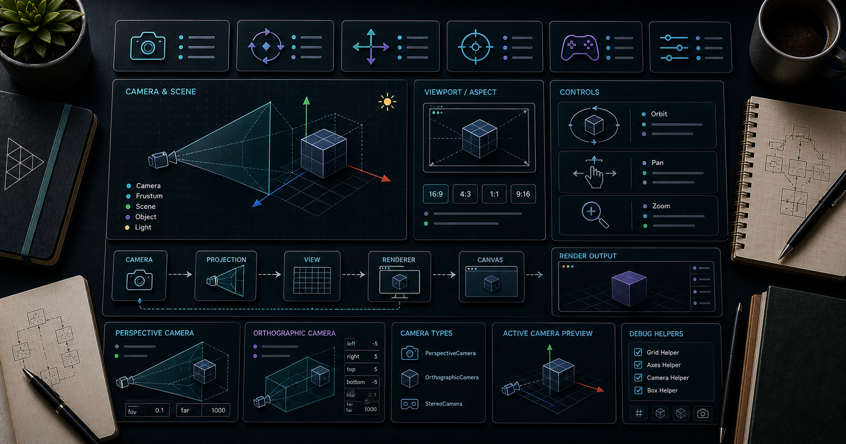
Three.js Course — 02 · Cameras, Controls, and Coordinate Systems
Camera defines what the user sees; controls let them navigate. Three.js ships several of each, and the right choice depends on the experience you want — a product viewer (OrbitControls), a first-person walker (PointerLockControls), a top-down map (MapControls), or a CAD-style turntable (TrackballControls). This post covers the camera types, the built-in controls, how the coordinate system works, and the most useful camera utilities (, frustum culling, raycasting from screen, helper visualisations).
> Series map: 00 Foundations → 01 Geometry & Materials → 02 Cameras & Controls (this post) → 03 Lighting & Shadows → 04 Textures & PBR → 05 Asset Pipeline → 06 Animation → 07 Instancing & Batching → 08 Low-End Perf → 09 Shaders → 10 Post-Processing → 11 Physics → 12 R3F → 13 AI 3D.
Learning Outcome
- Choose between and .- Tune FOV, near, far planes correctly.- Use , , , , , , .- Manipulate position + lookAt in world and local space.- Use helpers (, , ) for debugging.- Pick objects with a from a mouse click.
Chapter 1 — Coordinate system + units
Three.js uses a right-handed coordinate system with Y-up:
- Units are arbitrary — pick one (often metres for physics-friendly scenes) and stay consistent.- Default camera sits at the origin looking down .- A is centred at the local origin, sides of length 1.
> Trick: mismatched scales across imported assets (one in mm, one in m, one in inches) is the #1 "why is my model invisible / dust-sized" bug. Standardise the unit before importing. Most exporters offer a scale factor.
Chapter 2 — PerspectiveCamera
Mimics a real lens: distant objects appear smaller, parallel lines converge.
| Knob | Effect | Typical ||------|--------|---------|| | wider = more in frame, more "fish-eye" feel | 45-75 game; 25-35 cinematic || | match canvas size | || | nearer than this is clipped | 0.1 (units of metres ≈ 10 cm) || | further than this is clipped | 1000 |
The near/far depth problem
Depth buffer precision is non-linear — most precision is packed near the camera. A huge ratio (e.g., 0.001 / 10000 = 10⁷) causes z-fighting (flickering coplanar surfaces).
Rule: keep . If your scene needs both centimetre detail and kilometres of distance, use a logarithmic depth buffer: .
Update after change
Every time you change , , , or :
Chapter 3 — OrthographicCamera
Parallel projection — no perspective foreshortening. Used for 2D / isometric / CAD / minimaps.
To keep things sized correctly with the window, derive from the aspect ratio:
On resize:
Chapter 4 — lookAt + position
orients the camera; it doesn't move it. Call after setting position.
To follow a moving target every frame:
For smooth chase cameras, lerp position + lookAt:
Chapter 5 — Built-in controls
All controls live at and need the camera + the canvas DOM element.
| Controls | Feel | Typical use ||----------|------|--------------|| | orbit a target, dolly with scroll, pan with right-click | product viewers, scene exploration || | OrbitControls tuned for top-down maps — left-click pans | maps, terrain, 2.5D dashboards || | free orbit, no up-axis lock | CAD, scientific visualisation || | trackball with gizmo on screen | precise manipulation || | first-person mouse-look (locks pointer) | FPS games, walk-throughs || | WASD + mouse, no pointer lock | exploratory scenes || | 6-DoF flight | space scenes || | gizmo to translate/rotate/scale objects | editors, level builders || | click-drag objects across the screen plane | UI, prototypes |
OrbitControls (the everyday default)
repositions the orbit pivot. Useful to keep focus on a model whose centre is not at the origin.
PointerLockControls (FPS)
On Escape, the browser unlocks the pointer automatically. Combine with custom WASD logic to walk.
Chapter 6 — Helpers
For learning + debugging, the helpers visualise invisible state:
Strip these in production builds — they cost draw calls + memory.
Chapter 7 — Raycasting (picking objects)
To know what's under the mouse:
Performance tips for raycasting
- walks every triangle by default — slow with > 10k tris.- For large scenes, use a BVH (Bounding Volume Hierarchy): the three-mesh-bvh library accelerates raycasts up to 100× and reuses the BVH per geometry.- For purely UI hit-tests over flat icons, raycast against a low-poly invisible proxy mesh, not the full visual model.
Chapter 8 — Cameras inside a scene graph
A camera is an . You can add it to a group and the group's transforms cascade:
Useful for: FPS character rigs (move rig for body, rotate camera for look), AR camera mounts, cinematic camera tracks.
Chapter 9 — Multiple viewports
Render two views in one canvas (mini-map, picture-in-picture):
Each viewport gets its own camera but shares the scene.
Practice Exercises
Exercise 1 — OrbitControls + helpers
Scene with a cube, OrbitControls, AxesHelper, GridHelper. Orbit around, confirm axes and grid behave intuitively.
Exercise 2 — Orthographic isometric
Switch the camera to OrthographicCamera at . Render a few cubes. Note the isometric look.
Exercise 3 — Pick + recolour
Implement Chapter 7 raycasting. Click on any object → set its to red.
Exercise 4 — First-person walk
PointerLockControls + WASD. Spawn a few box "obstacles" on a plane. Walk around. (No collision yet — Post 11 covers physics.)
Exercise 5 — Chase camera
A small ball moves in a circle. The camera follows behind at fixed distance + slight elevation. Use for smoothing.
Exercise 6 — Minimap
Render the main scene from a perspective camera; in a 200×200 corner viewport render from a top-down orthographic camera. Sync them on each frame.
Cheat-sheet
| What | How ||------|-----|| Perspective camera | || Ortho camera | || After changing camera params | || Look at | (after setting position) || OrbitControls default | most use-cases || MapControls | top-down pannable || PointerLockControls | FPS feel || TransformControls | gizmo to move objects || Axes / grid helper | debugging || Raycaster | ; || BVH for raycast | library || Damping | + || Group with camera child | move rig, camera follows || Multiple viewports | + per render || Avoid z-fighting | keep ; or |
What's next
Post 03 covers lighting and shadows: light types, shadow maps (Basic / PCF / PCFSoft / VSM), cascaded shadow maps for big terrains, and the bias/normalBias tuning that decides whether your scene looks great or covered in artefacts.
References
- Three.js docs — Cameras- Three.js docs — Controls- three-mesh-bvh — fast raycasting + collision queries.- Three.js manual — Cameras- Three.js manual — Picking
> Note: this post is in progress. Planned additions: camera shake recipes, dolly-zoom (Hitchcock) effect, camera path animation via , VR camera in WebXR.
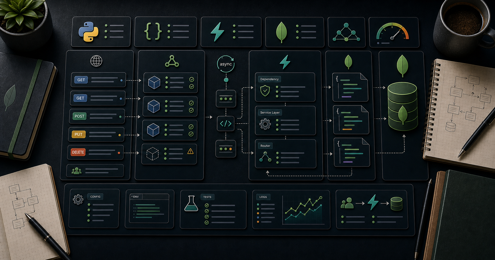
MongoDB Course — 19 · Beanie + Pydantic v2 + FastAPI — Async Python ODM
The Python equivalent of Mongoose in 2026 is Beanie — an async ODM built on Motor + Pydantic. It fits naturally into FastAPI (which is also Pydantic-based) and gives type-safe models, async I/O, validation, indexes, hooks, links (relations), aggregations, and migrations in one package. This post covers the working set: models, CRUD, indexes, links + back-links, hooks, projections, aggregations, transactions, integration patterns with FastAPI.
> Series map: 17 base course → 18 Mongoose deep → 19 Beanie + FastAPI (this post) → 20 Outbox → ... → 29 K8s + mongosync + cost.
Learning Outcome
- Set up Beanie + Motor with FastAPI lifespan.- Define models with Pydantic v2 + Indexed + relations ().- CRUD with type-safe queries.- Use projections + aggregations + bulk writes.- Hook into events (, ).- Use transactions inside Beanie.- Integrate with FastAPI dependency injection.
Chapter 1 — Install + connect
registers your models against the database and creates declared indexes. One call per process.
Chapter 2 — Models
Key elements:
- Inherit . auto-managed as ObjectId.- for index declarations.- inner class for collection name + index definitions.- / hooks similar to Mongoose middleware.- Pydantic v2 validators () run on construction + assignment.
Chapter 3 — CRUD
Query expressions use the Python operators on model fields — fully type-checked.
Chapter 4 — Indexes
Indexes created at . For production, disable + create via migrations (same advice as Mongoose Post 18).
Chapter 5 — Links (relations)
Beanie supports linked documents — equivalent to Mongoose :
Multi-level fetch supported. Like Mongoose populate, this issues additional queries — for hot endpoints prefer aggregation .
for reverse references (also fetched on demand).
Chapter 6 — Projections
Use for list endpoints — server returns only projected fields + Pydantic constructs the typed slim object.
Chapter 7 — Aggregations
Returns raw dicts. To get typed results, pass a :
For aggregation builders + type-safe pipeline construction, the community and helpers exist. Most teams just use dict pipelines as in mongosh.
Chapter 8 — Hooks (events)
Events: , , , , , . Multiple events per decorator. Async or sync function bodies.
Chapter 9 — Transactions
Or with retry helper from Motor (Post 09 patterns apply).
must be passed to every op — same rule as Mongoose + the official driver.
Chapter 10 — Bulk writes
Batches the operations into a single call — much faster than per-doc round-trips.
Chapter 11 — FastAPI integration patterns
Separation of concerns:
- — request body.- (Beanie) — database document.- — response body (no internal fields).
Helps avoid leaking server-side fields (, , etc.) into responses.
Dependency injection for repositories
Useful when you want to mock the repository in tests.
Chapter 12 — Migrations
Beanie has CLI:
Migration files apply schema-evolution + index changes idempotently. State stored in collection.
For complex schema versioning (Post 07), pair with on documents + lazy migration in app code.
Chapter 13 — Common pitfalls
| Pitfall | Cause | Fix ||---------|-------|-----|| called per request | overhead, leak risk | call once in lifespan || Links populate causing N+1 | many docs each | aggregation || Projection model field name mismatch | aliases needed | use || install error | missing optional dep | || Auto-index blocks on production startup | huge collection | disable + migrate manually || Mixed sync + async code | accidental blocking call | wrap with || Old Pydantic v1 examples | breaking changes | always use Pydantic v2 || vs confusion | Beanie exposes (the str-friendly view) | match docs |
Practice Exercises
Exercise 1 — Hello Beanie + FastAPI
Build the FastAPI skeleton in Chapter 1 + 2. Create model. POST + GET endpoint. Test with .
Exercise 2 — Aggregation
Build an endpoint that returns count per country via an aggregation projected to a Pydantic model.
Exercise 3 — Links
Create linking to . Insert a few. Endpoint returns the order with the linked user fetched.
Exercise 4 — Hooks
Add a hook to that sets and validates .
Exercise 5 — Bulk + transaction
Endpoint that inserts a batch of 100 users in a single . Wrap in a transaction (overkill for inserts; just to practice).
Exercise 6 — Migration
Add an migration. Run . Verify from mongosh shows it.
Cheat-sheet
| What | How ||------|-----|| Install | || Init | || Model | || Index | or || Query | (type-safe) || Insert | or || Update | (state-managed) or || Delete | || Project | || Aggregate | || Link | field; || Hook | / || Transaction | || Bulk | || FastAPI | lifespan to init/close; Pydantic models for request/response || Migration | / || Async only | use Motor under the hood |
What's next
Post 20 covers the outbox pattern + transactional event publishing via change streams — the canonical way to publish reliable events when mutating MongoDB inside a service.
References
- Beanie ODM docs- Beanie GitHub- Motor docs- Pydantic v2 docs- FastAPI docs
> Note: this post is in progress. Planned additions: Beanie + Strawberry GraphQL integration; ODMantic vs Beanie comparison; testing Beanie with Testcontainers (Post 25).

Three.js Course — 01 · Geometry & Materials
A mesh in Three.js is . Geometry defines the shape — a list of vertex positions, normals, UVs, and how they form triangles. Material defines how each pixel of the shape is shaded — colour, roughness, light response, transparency. This post covers , the built-in geometries, and the full material family from (no lighting at all) up to (full PBR with clearcoat, sheen, transmission, iridescence).
> Series map: 00 Foundations → 01 Geometry & Materials (this post) → 02 Cameras & Controls → 03 Lighting & Shadows → 04 Textures & PBR → 05 Asset Pipeline → 06 Animation → 07 Instancing & Batching → 08 Low-End Perf → 09 Shaders → 10 Post-Processing → 11 Physics → 12 R3F → 13 AI 3D.
Learning Outcome
- Build a from raw arrays of positions, normals, UVs, and indices.- Use the built-in geometries (Box, Sphere, Plane, Cylinder, Cone, Torus, TorusKnot, Tube, Lathe, Extrude, Text).- Distinguish the material families: Basic, Lambert, Phong, Standard, Physical, Toon, MatCap, Depth, Normal, Line, Sprite.- Understand which materials need lights and which don't.- Use wireframe, flat shading, double-sided rendering, and transparency.- Apply UV coordinates that make textures look right (Post 04 covers texture loading).
Chapter 1 — BufferGeometry: the low-level shape
Every geometry in Three.js is a . It's a container for arrays describing per-vertex data.
Attributes
| Attribute | Type | What ||-----------|------|------|| | Float32, 3 components | x, y, z of each vertex || | Float32, 3 components | surface normal (for lighting) || | Float32, 2 components | texture coordinates (0-1) || | Float32, 3 components | per-vertex tint (optional) || | Float32, 4 components | required for normal maps || | Uint16 / Uint32 | triangle vertex indices (optional) |
Build a triangle by hand
Direct array control is what you reach for when generating procedural geometry (terrain, ribbons, particles). For everyday primitives, use the built-ins.
Chapter 2 — Built-in geometries
| Class | Notes | Common args ||-------|-------|-------------|| | 6-face box | || | UV sphere | || | flat quad | || | flat disc | || | cylinder | || | cylinder w/ top = 0 | || | donut | || | mathematical knot | || , , , | platonic solids | || | sweep along a curve | || | revolution of a 2D profile | || | extrude a 2D shape into 3D | || | 3D text from a Font | — needs |
Subdivision matters
A is faceted; is smooth. Higher segments cost more vertices, more shading work, more memory. Profile in .
> Trick: when modelling stylised / low-poly art, low segment counts plus on the material gives the faceted look on purpose.
Chapter 3 — Material family
A material decides how each fragment (pixel) is shaded. The list, from cheapest to most expensive:
| Material | Lights needed? | Cost | When ||----------|----------------|------|------|| | no | very cheap | UI, sprites, "unlit" look || | n/a | cheap | shadows, depth visualisation || | no (encodes normals as RGB) | cheap | debugging, stylised || | no (uses a "material capture" image) | cheap | stylised — looks lit but isn't || | yes (diffuse only) | cheap | matte non-shiny surfaces || | yes (diffuse + specular) | medium | shiny non-PBR || | yes | medium | cel-shaded / cartoon || | yes | medium | PBR default — covered fully in Post 04 || | yes | high | PBR + clearcoat, sheen, transmission, iridescence, anisotropy || , | n/a | cheap | lines || | n/a | cheap | particles || | n/a | cheap | 2D billboards always facing camera || / / (TSL) | depends | depends | custom (Post 09) |
When each lights up
- Unlit family (, , , , , , ) ignore lights entirely — they render the same regardless of scene lighting.- Lit family (, , , , ) need at least one light in the scene; otherwise they appear black.
> Trick: a beginner's "it's just black" problem is almost always: lit material + no lights. Either add a / , or switch the material to while debugging.
Chapter 4 — MeshStandardMaterial (the modern default)
Physically-based rendering means: photons behave physically; a few intuitive parameters (, ) replace dozens of arbitrary knobs.
Post 04 covers the textures themselves.
Physical extensions
extends Standard with:
| Property | What ||----------|------|| , | car paint, varnished wood || , , | velvet, fabric softness || , , | glass-like refraction || , | thin-film effect (soap bubble, oil slick) || | brushed metal directional highlight || , | tinted glass |
Chapter 5 — Common material flags
DoubleSide cost
doubles the fragment shader work for that mesh — every triangle is rasterised twice (once per facing). Use only when needed (paper-thin objects, particle quads). For closed shapes, (default) is correct and faster.
Transparency caveats
Transparent objects must be sorted back-to-front for correct blending. Three.js does this per-mesh automatically ( by default). It cannot sort within a single mesh — long beard hair, foliage cards, particle clouds will exhibit artefacts. Workarounds:
1. instead of for binary cut-outs (no sorting needed).2. Separate meshes per leaf cluster (slow).3. Order-independent transparency (OIT) via custom shader (advanced).
Chapter 6 — Wireframe + flat shading recipes
Quick stylised looks without writing a shader:
is the right tool for "outline the silhouette of this object" without dotting every triangle.
Chapter 7 — Disposing geometry + materials
Three.js does not garbage-collect GPU resources automatically. When removing meshes:
Forgetting this in a long-running app causes GPU memory to climb until the tab crashes. Especially important when loading and unloading scenes / models.
A helper:
Practice Exercises
Exercise 1 — Built-in zoo
Render 6 objects in a row: Box, Sphere, Torus, TorusKnot, Cone, Icosahedron. Each with a different colour. Add ambient + directional light.
Exercise 2 — Compare materials
Same sphere, 5 copies side by side, each with a different material: Basic, Lambert, Phong, Standard, Physical (with ). Observe the difference.
Exercise 3 — Wireframe + flatShading combo
A low-poly icosahedron () with . Overlay an outline. Should look like a polygonal gemstone.
Exercise 4 — Procedural geometry
Build a of 100 random points ( material). Animate each point's position by a sine wave per frame. (Foreshadows particle systems and shaders.)
Exercise 5 — Disposal drill
In a loop, every 2 seconds: remove the current mesh from the scene and add a new sphere with random colour. Log to confirm it stays low when you dispose properly.
Cheat-sheet
| What | How ||------|-----|| Buffer geometry | + || Index | || Recompute normals | || Recompute tangents | (needs ) || Box / Sphere / Plane / Torus | etc. || Unlit | , , || Lit PBR | (default for new work) || Glass / car paint | + clearcoat / transmission || Cel-shaded | || Wireframe | (or use ) || Flat shading | || Double-sided | || Cut-out alpha | (no sorting needed) || Free GPU memory | + + |
What's next
Post 02 covers cameras, controls, and the coordinate system — what perspective vs orthographic actually do, the four built-in controls (Orbit, Map, Pointer-Lock, Trackball), and the math of + world-vs-local space.
References
- Three.js docs — BufferGeometry- Three.js docs — Materials- Three.js manual — Primitives- Three.js manual — Materials- Disposing objects in Three.js (forum)
> Note: this post is in progress. Planned additions: BufferGeometryUtils.mergeGeometries example; CSG (constructive solid geometry) via three-bvh-csg; signed-distance-field text intro.