Up to now a matrix has been a table of numbers that you multiply and row-reduce. This post changes the point of view: a matrix is only a description of a linear map, written in one particular pair of bases. Change the bases and the same map gets a different matrix. That idea explains why rank, trace and determinant are "real" properties of a map while individual entries are not, and it is the doorway to eigenvalues in the next post. The second half of the post builds the determinant from three simple rules, proves the key facts (product rule, invertibility test, Cramer's rule), and shows what the number means geometrically: the factor by which a map scales area or volume, with a sign for orientation.

Series map: 00 Vectors & Linear Systems → 01 Matrix Algebra, Inverses & LU → 02 Vector Spaces, Basis & Dimension → 03 Linear Maps, Change of Basis & Determinants (this post) → 04 Eigenvalues & Diagonalization → 05 Inner Products, Spectral Theorem & SVD.

Learning Outcome

Decide whether a given function between vector spaces is linear, and find its kernel and image.
State and prove the rank–nullity theorem for linear maps, and use it to relate injective, surjective and invertible.
Write the matrix of a linear map relative to any bases, and explain why composition of maps is the matrix product.
Convert coordinates between bases, and compute the matrix of a map in a new basis with $P^{-1}AP$ .
Recognise rotations, reflections, shears, projections and scalings in $\mathbb{R}^2$ from their matrices.
Define the determinant by its three axioms, compute it by cofactor expansion and by elimination, and prove $\det(AB) = \det A \det B$ .
Interpret $\lvert\det A\rvert$ as a volume scaling factor and the sign of $\det A$ as orientation.
Solve small systems with Cramer's rule, and explain why it is not used for large ones.

Chapter 1 — Linear maps

Terminology

Vector space $V$ over $\mathbb{R}$ — as in Linear Algebra 02: a set with addition and scalar multiplication obeying the eight axioms. Everything in this post also works over $\mathbb{C}$ or any field.
Linear map (linear transformation) $T: V \to W$ — a function that respects addition and scalar multiplication (definition below). When $V = W$ it is also called a linear operator on $V$ .
Domain $V$ and codomain $W$ — where inputs live and where outputs are allowed to land.
Kernel (null space) $\ker T = \{v \in V : T(v) = 0\}$ .
Image (range) $\operatorname{im} T = \{T(v) : v \in V\}$ .
Rank of $T$ — $\dim \operatorname{im} T$ . Nullity of $T$ — $\dim \ker T$ .
Injective (one-to-one) — $T(u) = T(v)$ implies $u = v$ . Surjective (onto) — $\operatorname{im} T = W$ . Bijective — both.
Isomorphism — a bijective linear map. $V$ and $W$ are isomorphic, written $V \cong W$ , if an isomorphism exists.
$P_n$ — polynomials of degree at most $n$ with real coefficients; $\dim P_n = n + 1$ .

Definition

A function $T: V \to W$ is linear if for all $u, v \in V$ and all scalars $c$ :

$T(u + v) = T(u) + T(v), \qquad T(cv) = c\,T(v).$

The two conditions combine into one: $T(c_1 v_1 + c_2 v_2) = c_1 T(v_1) + c_2 T(v_2)$ . By induction, a linear map sends every linear combination to the same combination of the images. Taking $c = 0$ gives $T(0) = 0$ : a linear map always sends zero to zero.

Examples:

Matrix maps. For an $m \times n$ matrix $A$ , the map $T_A: \mathbb{R}^n \to \mathbb{R}^m$ , $T_A(x) = Ax$ , is linear because $A(u+v) = Au + Av$ and $A(cv) = cAv$ (Linear Algebra 01).
Differentiation. $D: P_3 \to P_2$ , $D(p) = p'$ . The sum rule and the constant-multiple rule of calculus are exactly the two linearity conditions.
Integration. $I: C[0,1] \to \mathbb{R}$ , $I(f) = \int_0^1 f(x)\,dx$ , where $C[0,1]$ is the space of continuous functions on $[0,1]$ .
Evaluation. $E: P_2 \to \mathbb{R}^2$ , $E(p) = (p(0), p(1))$ .
Transpose. $M \mapsto M^T$ from $m \times n$ matrices to $n \times m$ matrices.

Non-examples:

Translation $T(x) = x + b$ with $b \neq 0$ : $T(0) = b \neq 0$ , so it is not linear. (It is called affine.)
$T(x, y) = (x + y, xy)$ : $T(2 \cdot (1,1)) = (4, 4)$ but $2\,T(1,1) = (4, 2)$ .
$T(x) = \lvert x\rvert$ on $\mathbb{R}$ : $T(-1) = 1 \neq -T(1)$ .

Trick: To show a map is not linear, one counterexample is enough — and checking $T(0) = 0$ first catches many cases in one line. To show a map is linear, you must check both conditions for arbitrary inputs.

A linear map is fixed by what it does to a basis

Theorem 1. Let $b_1, \dots, b_n$ be a basis of $V$ and let $w_1, \dots, w_n$ be any vectors in $W$ . There is exactly one linear map $T: V \to W$ with $T(b_i) = w_i$ for every $i$ .

Proof. Every $v \in V$ has unique coordinates: $v = c_1 b_1 + \dots + c_n b_n$ (Linear Algebra 02). Define $T(v) = c_1 w_1 + \dots + c_n w_n$ . This is well defined because the coordinates are unique. It is linear: if $v$ has coordinates $c_i$ and $u$ has coordinates $d_i$ , then $u + v$ has coordinates $c_i + d_i$ and $kv$ has coordinates $kc_i$ , and the formula is linear in the coordinates. It sends $b_i$ to $w_i$ . For uniqueness, any linear $S$ with $S(b_i) = w_i$ satisfies $S(v) = \sum c_i S(b_i) = \sum c_i w_i = T(v)$ . ∎

This theorem is the reason matrices work at all: to store a linear map you only need to store $n$ vectors, the images of the basis vectors.

Chapter 2 — Kernel, image and rank–nullity

Kernel and image are subspaces

Proposition 2. For linear $T: V \to W$ , $\ker T$ is a subspace of $V$ and $\operatorname{im} T$ is a subspace of $W$ .

Proof. $T(0) = 0$ , so $0$ is in both. If $T(u) = T(v) = 0$ then $T(u + cv) = 0 + c \cdot 0 = 0$ , so the kernel is closed under addition and scaling. If $w_1 = T(v_1)$ and $w_2 = T(v_2)$ then $w_1 + c w_2 = T(v_1 + c v_2)$ is also in the image. ∎

For a matrix map $T_A$ , the kernel is the null space $N(A)$ and the image is the column space $C(A)$ from Linear Algebra 02.

Proposition 3. $T$ is injective if and only if $\ker T = \{0\}$ .

Proof. If $T$ is injective and $T(v) = 0 = T(0)$ , then $v = 0$ . Conversely, if $\ker T = \{0\}$ and $T(u) = T(v)$ , then $T(u - v) = 0$ , so $u - v = 0$ . ∎

Watch out: "The only solution of $T(v) = 0$ is $v = 0$ " is a statement about one equation, but it controls every equation $T(v) = w$ : each one then has at most one solution. This is the map version of "no free variables" from Linear Algebra 00.

Rank–nullity for linear maps

Linear Algebra 02 proved $\operatorname{rank} A + \dim N(A) = n$ for an $m \times n$ matrix by counting pivot and free columns. Here is the version for maps, with a proof that uses no matrices at all.

Theorem 4 (rank–nullity). Let $V$ be finite-dimensional and $T: V \to W$ linear. Then $\operatorname{im} T$ is finite-dimensional and

$\dim V = \dim \ker T + \dim \operatorname{im} T.$

Proof. $\ker T$ is a subspace of the finite-dimensional space $V$ , so it has a basis $u_1, \dots, u_k$ (possibly $k = 0$ ). By the basis-extension theorem of Linear Algebra 02, extend it to a basis $u_1, \dots, u_k, w_1, \dots, w_r$ of $V$ , so $\dim V = k + r$ . We show that $T(w_1), \dots, T(w_r)$ is a basis of $\operatorname{im} T$ ; then $\dim \operatorname{im} T = r$ and we are done.

Spanning. Any vector in the image is $T(v)$ for some $v = \sum a_i u_i + \sum b_j w_j$ . Since $T(u_i) = 0$ , we get $T(v) = \sum b_j T(w_j)$ .

Independence. Suppose $\sum c_j T(w_j) = 0$ . Then $T\left(\sum c_j w_j\right) = 0$ , so $\sum c_j w_j \in \ker T$ and can be written as $\sum d_i u_i$ . Then $\sum c_j w_j - \sum d_i u_i = 0$ is a linear relation among the basis vectors of $V$ , so every $c_j$ (and every $d_i$ ) is zero. ∎

Worked example. $T: \mathbb{R}^3 \to \mathbb{R}^2$ , $T(x, y, z) = (x + 2y - z,\ 2x + 4y + z)$ . Its matrix is

$A = \begin{pmatrix} 1 & 2 & -1 \\ 2 & 4 & 1 \end{pmatrix}.$

Solving $T(v) = 0$ : adding the two equations gives $3x + 6y = 0$ , so $x = -2y$ , and then $z = x + 2y = 0$ . The kernel is the line spanned by $(-2, 1, 0)$ , so the nullity is 1. Rank–nullity forces $\dim \operatorname{im} T = 3 - 1 = 2$ , so the image is all of $\mathbb{R}^2$ : $T$ is surjective but not injective.

Worked example (no matrix in sight). $D: P_3 \to P_2$ , $D(p) = p'$ . The kernel is the constant polynomials (dimension 1). Every $q \in P_2$ is the derivative of some cubic, so the image is $P_2$ (dimension 3). Check: $4 = 1 + 3$ .

Consequences

Corollary 5. Let $T: V \to W$ be linear with $V, W$ finite-dimensional.

If $\dim V > \dim W$ , then $T$ is not injective (the kernel has dimension at least $\dim V - \dim W > 0$ ).
If $\dim V < \dim W$ , then $T$ is not surjective (the image has dimension at most $\dim V$ ).
If $\dim V = \dim W$ , then $T$ injective $\iff$ $T$ surjective $\iff$ $T$ is an isomorphism.

Proof of 3. Injective means $\dim \ker T = 0$ , which by rank–nullity means $\dim \operatorname{im} T = \dim V = \dim W$ , which means $\operatorname{im} T = W$ (a subspace of full dimension is the whole space). ∎

Part 3 is the abstract form of the invertible matrix theorem from Linear Algebra 01: for a square matrix, "only the trivial solution" and "a solution for every right-hand side" are the same condition.

Theorem 6 (classification by dimension). Two finite-dimensional spaces are isomorphic if and only if they have the same dimension. In particular every $n$ -dimensional real space is isomorphic to $\mathbb{R}^n$ .

Proof. An isomorphism sends a basis to a basis (it is injective, so independence is kept, and surjective, so the images span), so dimensions agree. Conversely, if $\dim V = n$ with basis $b_1, \dots, b_n$ , the coordinate map $v \mapsto (c_1, \dots, c_n)$ is linear, injective and surjective. Composing two such maps gives $V \cong \mathbb{R}^n \cong W$ . ∎

The inverse of an isomorphism is automatically linear: if $T(u') = u$ and $T(v') = v$ , then $T(u' + cv') = u + cv$ , so $T^{-1}(u + cv) = T^{-1}(u) + cT^{-1}(v)$ .

Common pitfall: Isomorphic does not mean equal. $P_2$ and $\mathbb{R}^3$ are isomorphic, but the isomorphism depends on a choice of basis. There is no single "correct" identification — which is exactly why the next chapter keeps track of bases.

Chapter 3 — The matrix of a linear map

Coordinates

Fix an ordered basis $\mathcal{B} = (b_1, \dots, b_n)$ of $V$ . The coordinate vector of $v$ is the column $[v]_{\mathcal{B}} = (c_1, \dots, c_n)^T$ with $v = \sum c_i b_i$ . The map $v \mapsto [v]_{\mathcal{B}}$ is the isomorphism $V \to \mathbb{R}^n$ of Theorem 6. Order matters: swapping $b_1$ and $b_2$ swaps the first two coordinates.

The matrix relative to two bases

Let $T: V \to W$ be linear, with basis $\mathcal{B} = (b_1, \dots, b_n)$ of $V$ and $\mathcal{C} = (c_1, \dots, c_m)$ of $W$ . The matrix of $T$ relative to $\mathcal{B}$ and $\mathcal{C}$ is the $m \times n$ matrix

$[T]_{\mathcal{C} \leftarrow \mathcal{B}} = \Big( [T(b_1)]_{\mathcal{C}} \ \ [T(b_2)]_{\mathcal{C}} \ \ \cdots \ \ [T(b_n)]_{\mathcal{C}} \Big).$

Column $j$ = the $\mathcal{C}$ -coordinates of the image of the $j$ -th basis vector. With it, applying $T$ becomes matrix multiplication on coordinates:

$[T(v)]_{\mathcal{C}} = [T]_{\mathcal{C} \leftarrow \mathcal{B}}\, [v]_{\mathcal{B}}.$

Why: if $v = \sum x_j b_j$ then $T(v) = \sum x_j T(b_j)$ , and taking $\mathcal{C}$ -coordinates (a linear operation) gives $\sum x_j [T(b_j)]_{\mathcal{C}}$ , which is the matrix times the column $x$ .

The arrow notation $\mathcal{C} \leftarrow \mathcal{B}$ reads right to left: coordinates in $\mathcal{B}$ go in, coordinates in $\mathcal{C}$ come out. When $V = W$ and the same basis is used on both sides, write $[T]_{\mathcal{B}}$ .

Worked example. $D: P_3 \to P_2$ with bases $(1, x, x^2, x^3)$ and $(1, x, x^2)$ . The images of the basis vectors are $0,\ 1,\ 2x,\ 3x^2$ , whose coordinates are the columns:

$[D] = \begin{pmatrix} 0 & 1 & 0 & 0 \\ 0 & 0 & 2 & 0 \\ 0 & 0 & 0 & 3 \end{pmatrix}.$

Check with $p = 1 + 2x - x^2 + 4x^3$ : $[D]\,(1, 2, -1, 4)^T = (2, -2, 12)^T$ , and indeed $p' = 2 - 2x + 12x^2$ . The matrix has rank 3 and a one-dimensional null space spanned by $(1,0,0,0)^T$ — the constant polynomial 1 — matching the rank–nullity count above.

Composition is the matrix product

Theorem 7. Let $T: U \to V$ and $S: V \to W$ be linear, with bases $\mathcal{B}, \mathcal{C}, \mathcal{D}$ of $U, V, W$ . Then

$[S \circ T]_{\mathcal{D} \leftarrow \mathcal{B}} = [S]_{\mathcal{D} \leftarrow \mathcal{C}}\ [T]_{\mathcal{C} \leftarrow \mathcal{B}}.$

Proof. For every $u \in U$ : $[S(T(u))]_{\mathcal{D}} = [S]\,[T(u)]_{\mathcal{C}} = [S]\,[T]\,[u]_{\mathcal{B}}$ . Taking $u = b_j$ (so $[u]_{\mathcal{B}}$ is the $j$ -th standard column) shows that column $j$ of $[S \circ T]$ equals column $j$ of $[S][T]$ . ∎

This is why matrix multiplication is defined the strange row-times-column way: it is the only definition that makes "do $T$ , then do $S$ " correspond to a product. It also explains why the product is associative (composition of functions is) and generally not commutative (doing things in a different order usually gives a different result). The order is right to left: in $ST$ , $T$ acts first.

Two consequences follow at once. $T$ is an isomorphism if and only if its matrix (in any bases) is invertible, and then $[T^{-1}]_{\mathcal{B} \leftarrow \mathcal{C}} = \left([T]_{\mathcal{C} \leftarrow \mathcal{B}}\right)^{-1}$ . And the rank of $T$ equals the rank of any matrix that represents it.

Chapter 4 — Change of basis and similarity

The change-of-basis matrix

Let $\mathcal{E}$ be the standard basis of $\mathbb{R}^n$ and $\mathcal{B} = (b_1, \dots, b_n)$ another basis. Put the new basis vectors, written in standard coordinates, into the columns of

$P = P_{\mathcal{E} \leftarrow \mathcal{B}} = \big( b_1 \ \ b_2 \ \ \cdots \ \ b_n \big).$

Then $v = \sum c_i b_i = P\,[v]_{\mathcal{B}}$ , that is

$[v]_{\mathcal{E}} = P\,[v]_{\mathcal{B}}, \qquad [v]_{\mathcal{B}} = P^{-1}[v]_{\mathcal{E}}.$

$P$ is invertible because its columns are a basis. $P$ is simply the matrix of the identity map, $[\mathrm{id}]_{\mathcal{E} \leftarrow \mathcal{B}}$ : it takes $\mathcal{B}$ -coordinates in and gives $\mathcal{E}$ -coordinates out.

Common pitfall: The matrix whose columns are the new basis vectors converts new coordinates to old, not old to new. To get new coordinates you must solve $P c = v$ (or apply $P^{-1}$ ). Writing the arrow $\mathcal{E} \leftarrow \mathcal{B}$ on every change-of-basis matrix prevents this mistake.

The same map in a new basis

Let $T: \mathbb{R}^n \to \mathbb{R}^n$ have standard matrix $A = [T]_{\mathcal{E}}$ . Its matrix in the basis $\mathcal{B}$ is found by composing: convert $\mathcal{B}$ -coordinates to standard ( $P$ ), apply $T$ ( $A$ ), convert back ( $P^{-1}$ ):

$[T]_{\mathcal{B}} = P^{-1} A P.$

This is Theorem 7 applied to $T = \mathrm{id} \circ T \circ \mathrm{id}$ . For a map between different spaces, with change-of-basis matrices $P$ on the domain and $Q$ on the codomain, the rule is $[T]_{\mathcal{C}' \leftarrow \mathcal{B}'} = Q^{-1}\,[T]_{\mathcal{C} \leftarrow \mathcal{B}}\,P$ .

Worked example. Let $A = \begin{pmatrix} 2 & 1 \\ 1 & 2 \end{pmatrix}$ and take the basis $b_1 = (1, 1)$ , $b_2 = (1, -1)$ . Then

$P = \begin{pmatrix} 1 & 1 \\ 1 & -1 \end{pmatrix}, \quad P^{-1} = \frac{1}{2}\begin{pmatrix} 1 & 1 \\ 1 & -1 \end{pmatrix}, \quad P^{-1}AP = \begin{pmatrix} 3 & 0 \\ 0 & 1 \end{pmatrix}.$

You can see the diagonal answer directly: $Ab_1 = (3, 3) = 3b_1$ and $Ab_2 = (1, -1) = b_2$ . In the new basis the map just stretches the $b_1$ direction by 3 and leaves the $b_2$ direction alone. Now track one vector. $v = (5, 1)$ has $[v]_{\mathcal{B}} = P^{-1}v = (3, 2)$ , because $3(1,1) + 2(1,-1) = (5, 1)$ . In new coordinates the map gives $\operatorname{diag}(3,1)\,(3,2)^T = (9, 2)^T$ , and $9(1,1) + 2(1,-1) = (11, 7) = Av$ . The two routes agree.

Choosing a basis that makes the matrix diagonal is the whole subject of Linear Algebra 04: $b_1$ and $b_2$ here are eigenvectors.

Similarity

Square matrices $A$ and $B$ are similar if $B = P^{-1}AP$ for some invertible $P$ . Similar matrices are the same linear operator written in two bases. Similarity is an equivalence relation (reflexive with $P = I$ , symmetric with $P^{-1}$ , transitive with $PQ$ ).

Anything defined for the operator rather than the table of numbers must be the same for similar matrices. Such quantities are called similarity invariants:

Invariant	Why it survives $A \mapsto P^{-1}AP$
Rank	rank of the map, which does not depend on coordinates
Trace	$\operatorname{tr}(XY) = \operatorname{tr}(YX)$ , so $\operatorname{tr}(P^{-1}(AP)) = \operatorname{tr}((AP)P^{-1})$
Determinant	product rule (Chapter 6): $\det P^{-1} \det A \det P = \det A$
Characteristic polynomial, eigenvalues	Linear Algebra 04

The trace identity is a one-line calculation: $\operatorname{tr}(XY) = \sum_i \sum_j x_{ij} y_{ji} = \sum_j \sum_i y_{ji} x_{ij} = \operatorname{tr}(YX)$ . Check the example: $\operatorname{tr}A = 4 = 3 + 1$ .

Watch out: Equal invariants do not prove similarity. $I = \begin{pmatrix} 1 & 0 \\ 0 & 1\end{pmatrix}$ and $\begin{pmatrix} 1 & 1 \\ 0 & 1\end{pmatrix}$ have the same rank, trace and determinant, but only $I$ is similar to $I$ (because $P^{-1}IP = I$ for every $P$ ).

Chapter 5 — Geometry of maps in the plane

The quickest way to read a $2 \times 2$ matrix: its columns are where $e_1 = (1,0)$ and $e_2 = (0,1)$ land. Draw those two arrows and you have drawn the map, because the unit square goes to the parallelogram they span and every grid line goes to a parallel grid line.

Map	Matrix	What it does	det
Rotation by $\theta$	$\begin{pmatrix} \cos\theta & -\sin\theta \\ \sin\theta & \cos\theta \end{pmatrix}$	turns every vector by angle $\theta$ counter-clockwise	$1$
Reflection in the line at angle $\theta$	$\begin{pmatrix} \cos 2\theta & \sin 2\theta \\ \sin 2\theta & -\cos 2\theta \end{pmatrix}$	mirror image; vectors on the line stay put	$-1$
Shear	$\begin{pmatrix} 1 & k \\ 0 & 1 \end{pmatrix}$	slides each point sideways by $k$ times its height	$1$
Projection onto the line at angle $\theta$	$\begin{pmatrix} \cos^2\theta & \cos\theta\sin\theta \\ \cos\theta\sin\theta & \sin^2\theta \end{pmatrix}$	drops each point perpendicularly onto the line	$0$
Scaling	$\begin{pmatrix} a & 0 \\ 0 & b \end{pmatrix}$	stretches $x$ by $a$ and $y$ by $b$	$ab$

Where these come from:

Rotation. $e_1$ goes to $(\cos\theta, \sin\theta)$ and $e_2$ (at angle $90°$ ) goes to $(\cos(\theta + 90°), \sin(\theta + 90°)) = (-\sin\theta, \cos\theta)$ . For $\theta = 30°$ this gives $\begin{pmatrix} \sqrt{3}/2 & -1/2 \\ 1/2 & \sqrt{3}/2 \end{pmatrix}$ .
Projection. With the unit vector $u = (\cos\theta, \sin\theta)$ along the line, the projection of $x$ is $(u \cdot x)\,u = (u u^T) x$ , and $uu^T$ is the matrix in the table. It satisfies $P^2 = P$ : projecting twice is the same as projecting once.
Reflection. Reflection = $2 \times$ projection $-$ identity (go to the line, then the same distance again). Using $2\cos^2\theta - 1 = \cos 2\theta$ and $2\sin\theta\cos\theta = \sin 2\theta$ gives the table entry. It satisfies $F^2 = I$ .

Composition does not commute. Let $R$ be rotation by $90°$ and $F$ reflection in the $x$ -axis:

$R = \begin{pmatrix} 0 & -1 \\ 1 & 0 \end{pmatrix}, \quad F = \begin{pmatrix} 1 & 0 \\ 0 & -1 \end{pmatrix}, \quad FR = \begin{pmatrix} 0 & -1 \\ -1 & 0 \end{pmatrix}, \quad RF = \begin{pmatrix} 0 & 1 \\ 1 & 0 \end{pmatrix}.$

"Rotate, then reflect" ( $FR$ ) is the reflection in the line $y = -x$ ; "reflect, then rotate" ( $RF$ ) is the reflection in $y = x$ . Two different maps.

A projection is diagonal in the right basis. The projection onto the line $y = 2x$ has standard matrix $\frac{1}{5}\begin{pmatrix} 1 & 2 \\ 2 & 4 \end{pmatrix}$ . In the basis $(1, 2), (-2, 1)$ — one vector along the line, one perpendicular to it — its matrix is $\begin{pmatrix} 1 & 0 \\ 0 & 0 \end{pmatrix}$ : keep the first coordinate, kill the second. Same map, much clearer matrix.

Chapter 6 — The determinant

Terminology

Multilinear (in the rows) — linear in each row separately when the other rows are held fixed.
Alternating — the value is $0$ whenever two rows are equal.
Permutation of $\{1, \dots, n\}$ — a bijection $\sigma$ of the set to itself; $S_n$ is the set of all $n!$ of them.
Sign $\operatorname{sgn}(\sigma)$ — $+1$ if $\sigma$ is a product of an even number of swaps, $-1$ if odd. Equivalently $(-1)^{\text{number of inversions}}$ , where an inversion is a pair $i < j$ with $\sigma(i) > \sigma(j)$ .
Minor $M_{ij}$ — the determinant of the $(n-1) \times (n-1)$ matrix left after deleting row $i$ and column $j$ . Cofactor $C_{ij} = (-1)^{i+j} M_{ij}$ .

The three axioms

For $2 \times 2$ matrices you know $\det \begin{pmatrix} a & b \\ c & d \end{pmatrix} = ad - bc$ . The clean way to generalise is not to guess a formula but to list the properties we want and prove that exactly one function has them.

A function $D$ from $n \times n$ matrices to $\mathbb{R}$ is a determinant function if:

(Multilinear) $D$ is linear in each row: $D(\dots, u + cv, \dots) = D(\dots, u, \dots) + c\,D(\dots, v, \dots)$ , other rows fixed.
(Alternating) $D(A) = 0$ if two rows of $A$ are equal.
(Normalised) $D(I) = 1$ .

Theorem 8 (existence and uniqueness). There is exactly one determinant function, written $\det$ . Moreover, any function $D$ satisfying axioms 1 and 2 (but not necessarily 3) equals $D(I) \cdot \det$ .

Existence is shown by checking that the Leibniz formula below satisfies the three axioms; uniqueness follows because the axioms alone determine the value on every matrix, as the row-operation rules show. A full proof is in Axler (Chapter 9) or Hoffman and Kunze (Chapter 5); here we state it and use it.

What the axioms force: row operations

From the axioms alone:

Swapping two rows changes the sign. Put $u + v$ in both rows $i$ and $j$ . By axiom 2 the value is 0; expanding with axiom 1 gives $D(u,u) + D(u,v) + D(v,u) + D(v,v) = 0$ (other rows omitted), and the first and last terms are 0, so $D(u,v) = -D(v,u)$ .
Scaling one row by $c$ multiplies the determinant by $c$ (axiom 1).
Adding a multiple of one row to another leaves the determinant unchanged: $D(\dots, u + cv, \dots, v, \dots) = D(\dots, u, \dots, v, \dots) + c\,D(\dots, v, \dots, v, \dots)$ , and the last term is 0.
A zero row gives determinant 0 (scale that row by 0).
A triangular matrix has determinant = product of its diagonal entries. If all diagonal entries are nonzero, row replacements clear the off-diagonal entries without changing $D$ , leaving a diagonal matrix, and axiom 1 plus axiom 3 give the product. If a diagonal entry is zero, elimination produces a zero row, so both sides are 0.

These rules are also the fastest way to compute: row-reduce to triangular form, keeping track of swaps and scalings.

Leibniz formula and cofactor expansion

Leibniz formula.

$\det A = \sum_{\sigma \in S_n} \operatorname{sgn}(\sigma)\, a_{1\sigma(1)}\, a_{2\sigma(2)} \cdots a_{n\sigma(n)}.$

Each term picks one entry from every row and every column. For $n = 2$ there are two terms, $a_{11}a_{22} - a_{12}a_{21}$ . For $n = 3$ there are six:

$\det A = a_{11}a_{22}a_{33} + a_{12}a_{23}a_{31} + a_{13}a_{21}a_{32} - a_{13}a_{22}a_{31} - a_{11}a_{23}a_{32} - a_{12}a_{21}a_{33}.$

Cofactor (Laplace) expansion along row $i$ or column $j$ :

$\det A = \sum_{j=1}^{n} a_{ij} C_{ij} \quad \text{(row } i\text{)}, \qquad \det A = \sum_{i=1}^{n} a_{ij} C_{ij} \quad \text{(column } j\text{)}.$

The signs $(-1)^{i+j}$ follow a checkerboard starting with $+$ in the top-left corner. Expand along the row or column with the most zeros.

Worked example — three ways. Let

$M = \begin{pmatrix} 1 & 2 & 3 \\ 4 & 5 & 6 \\ 7 & 8 & 10 \end{pmatrix}.$

Cofactor expansion along row 1:

$\det M = 1(5 \cdot 10 - 6 \cdot 8) - 2(4 \cdot 10 - 6 \cdot 7) + 3(4 \cdot 8 - 5 \cdot 7) = 1(2) - 2(-2) + 3(-3) = -3.$

Leibniz, six terms: $50 + 84 + 96 - 105 - 48 - 80 = 230 - 233 = -3$ .

Elimination: $R_2 - 4R_1$ and $R_3 - 7R_1$ give rows $(0, -3, -6)$ and $(0, -6, -11)$ ; then $R_3 - 2R_2$ gives $(0, 0, 1)$ . Only row replacements were used, so the determinant is unchanged: $\det M = 1 \cdot (-3) \cdot 1 = -3$ .

Watch out: The "diagonals" trick (rule of Sarrus) works for $3 \times 3$ matrices only. For $4 \times 4$ it gives 8 terms, but the determinant has $4! = 24$ .

The product rule and other properties

Theorem 9. $\det(AB) = \det A \cdot \det B$ for all $n \times n$ matrices $A, B$ .

Proof. Fix $B$ and define $D(A) = \det(AB)$ . Row $i$ of $AB$ is (row $i$ of $A$ ) $\times B$ , which is linear in row $i$ of $A$ , so $D$ is multilinear in the rows of $A$ . If $A$ has two equal rows, so does $AB$ , so $D(A) = 0$ . By the second part of Theorem 8, $D(A) = D(I)\det A = \det(B)\det(A)$ . ∎

Theorem 10. $\det A^T = \det A$ .

Reason. In the Leibniz formula, the term for $\sigma$ in $\det A^T$ is the term for $\sigma^{-1}$ in $\det A$ , and $\operatorname{sgn}(\sigma^{-1}) = \operatorname{sgn}(\sigma)$ . As $\sigma$ runs over $S_n$ so does $\sigma^{-1}$ . ∎

So every statement about rows also holds for columns: column swaps flip the sign, and so on.

Theorem 11 (the invertibility test). A square matrix $A$ is invertible if and only if $\det A \neq 0$ . In that case $\det(A^{-1}) = 1/\det A$ .

Proof. Row-reduce: $E_k \cdots E_1 A = R$ with $R$ in reduced row echelon form. Each elementary operation multiplies the determinant by a nonzero number ( $-1$ , $c \neq 0$ , or $1$ ), so $\det A \neq 0 \iff \det R \neq 0$ . A square RREF is either $I$ (determinant 1) or has a zero row (determinant 0), and $R = I$ exactly when $A$ is invertible (Linear Algebra 01). For the formula, $\det A \det A^{-1} = \det I = 1$ . ∎

Further consequences:

$\det(cA) = c^n \det A$ for an $n \times n$ matrix (each of the $n$ rows is scaled). For the matrix $M$ above, $\det(2M) = 8 \cdot (-3) = -24$ .
Similar matrices have equal determinants, so $\det T$ is well defined for a linear operator $T$ : use its matrix in any basis.
For block upper triangular matrices, $\det \begin{pmatrix} A & B \\ 0 & D \end{pmatrix} = \det A \det D$ (with $A$ , $D$ square).

Common pitfall: $\det(A + B) \neq \det A + \det B$ in general. Try $A = B = I_2$ : the left side is $\det(2I) = 4$ , the right side is 2. The determinant is multiplicative, not additive.

Determinant as signed volume

For $n \times n$ $A$ with columns $a_1, \dots, a_n$ , the number $\lvert\det A\rvert$ is the volume (area when $n = 2$ ) of the parallelepiped $\{t_1 a_1 + \dots + t_n a_n : 0 \le t_i \le 1\}$ .

Why this is plausible: signed volume, as a function of the edge vectors, satisfies the axioms. Scaling one edge by $c$ scales the volume by $c$ . Sliding one edge along another (a shear) does not change the volume — Cavalieri's principle, the same reason a slanted stack of coins has the same volume as a straight one. Two equal edges give a flat box of volume 0. The unit cube has volume 1. By uniqueness, signed volume is the determinant.

Since $A$ sends the unit cube (volume 1) to this parallelepiped, and the map is linear, $A$ multiplies the volume of every region by $\lvert\det A\rvert$ . This is the factor $\lvert\det J\rvert$ in the change-of-variables formula for multiple integrals. The sign records orientation: $\det A > 0$ keeps the order of the edges (counter-clockwise stays counter-clockwise in the plane), $\det A < 0$ reverses it, as a mirror does. $\det A = 0$ means the space is flattened into a lower dimension — and that information cannot be undone, which is Theorem 11 seen geometrically.

Example in $\mathbb{R}^3$ : the columns $(1,0,0)$ , $(1,2,0)$ , $(1,1,3)$ form an upper triangular matrix with determinant $1 \cdot 2 \cdot 3 = 6$ , so the box they span has volume 6.

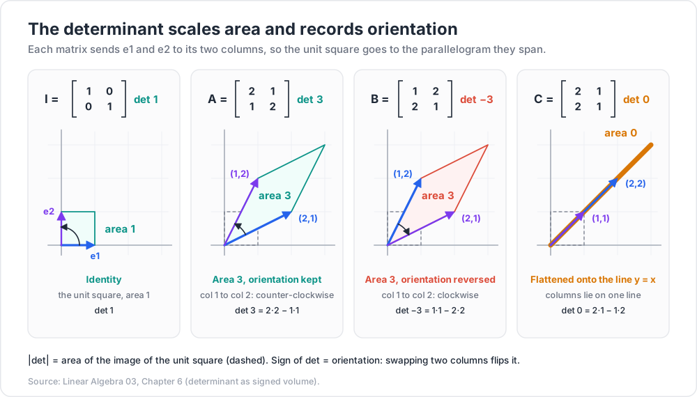
Four panels: the unit square with area 1; its image under A with columns (2,1) and (1,2), a parallelogram of area 3 with orientation kept (det 3); its image under B with columns (1,2) and (2,1), the same parallelogram with orientation reversed (det -3); and its image under C with columns (2,2) and (1,1), flattened onto the line y = x (det 0).

The figure uses $A = \begin{pmatrix} 2 & 1 \\ 1 & 2 \end{pmatrix}$ ( $\det = 3$ ), the same matrix with its columns swapped, $B = \begin{pmatrix} 1 & 2 \\ 2 & 1 \end{pmatrix}$ ( $\det = -3$ ), and $C = \begin{pmatrix} 2 & 1 \\ 2 & 1 \end{pmatrix}$ ( $\det = 0$ ). $A$ and $B$ produce the same parallelogram, but in $B$ the image of $e_1$ has moved to the other side of the image of $e_2$ : the turn from the first column to the second is clockwise, so the orientation is reversed. That is the column-swap rule, drawn.

Chapter 7 — Cramer's rule and the adjugate

Theorem 12 (Cramer's rule). If $\det A \neq 0$ , the unique solution of $Ax = b$ is

$x_i = \frac{\det A_i(b)}{\det A}, \qquad i = 1, \dots, n,$

where $A_i(b)$ is $A$ with column $i$ replaced by $b$ .

Proof. Let $I_i(x)$ be the identity matrix with column $i$ replaced by $x$ . Then $A\,I_i(x) = A_i(b)$ : its columns are $Ae_1, \dots, Ax, \dots, Ae_n$ , which are the columns of $A$ with $b = Ax$ in position $i$ . Expanding $\det I_i(x)$ along row $i$ gives $x_i$ . The product rule then gives $\det A \cdot x_i = \det A_i(b)$ . ∎

Worked example. $2x + y = 5$ , $x + 3y = 10$ . Here $\det A = 6 - 1 = 5$ , and

$x = \frac{\det\begin{pmatrix} 5 & 1 \\ 10 & 3 \end{pmatrix}}{5} = \frac{5}{5} = 1, \qquad y = \frac{\det\begin{pmatrix} 2 & 5 \\ 1 & 10 \end{pmatrix}}{5} = \frac{15}{5} = 3.$

Check: $2 + 3 = 5$ and $1 + 9 = 10$ .

The adjugate. Applying Cramer's rule to each column of $AX = I$ gives an explicit inverse:

$A^{-1} = \frac{1}{\det A}\operatorname{adj}(A), \qquad \operatorname{adj}(A)_{ij} = C_{ji}.$

Note the transpose: entry $(i,j)$ of the adjugate is the cofactor at $(j,i)$ . For $2 \times 2$ this is the familiar $\begin{pmatrix} a & b \\ c & d \end{pmatrix}^{-1} = \frac{1}{ad - bc}\begin{pmatrix} d & -b \\ -c & a \end{pmatrix}$ . For $M$ above,

$\operatorname{adj}(M) = \begin{pmatrix} 2 & 4 & -3 \\ 2 & -11 & 6 \\ -3 & 6 & -3 \end{pmatrix}, \qquad M^{-1} = -\frac{1}{3}\operatorname{adj}(M) = \begin{pmatrix} -2/3 & -4/3 & 1 \\ -2/3 & 11/3 & -2 \\ 1 & -2 & 1 \end{pmatrix}.$

Why not Cramer for large systems

Cramer's rule is valuable for theory: it shows that each $x_i$ is a rational function of the entries of $A$ and $b$ , so the solution depends continuously (indeed smoothly) on the data wherever $\det A \neq 0$ . As an algorithm it is a bad choice:

The Leibniz formula has $n!$ terms. For $n = 20$ that is $20! = 2\,432\,902\,008\,176\,640\,000 \approx 2.4 \times 10^{18}$ products for a single determinant.
Even computing each determinant by elimination, Cramer needs $n + 1$ determinants, each costing about as much as one full LU factorisation ( $\approx \tfrac{2}{3}n^3$ flops). Gaussian elimination solves the system with one factorisation.
Determinants are poor measures of numerical trouble. $\det(0.1\,I_{100}) = 10^{-100}$ , yet $0.1\,I$ is perfectly well-behaved. Closeness to singularity is measured by the condition number (Linear Algebra 05 and the planned numerical post), not by the size of $\det A$ .

Trick: In practice, a determinant is computed from an LU factorisation with partial pivoting, $PA = LU$ : $\det A = \pm \prod u_{ii}$ , the sign coming from the number of row swaps. This is exactly the elimination method above.

Practice Exercises

1. Which of these are linear? (a) $T: P_2 \to P_2$ , $T(p)(x) = p(x + 1)$ . (b) $T: \mathbb{R}^2 \to \mathbb{R}^2$ , $T(x, y) = (x + y, xy)$ . For the linear one, write its matrix in the basis $(1, x, x^2)$ and decide whether it is invertible.

Solution

(a) Linear: $(p + cq)(x + 1) = p(x+1) + c\,q(x+1)$ . The images of the basis are $1$ , $x + 1$ , $(x+1)^2 = 1 + 2x + x^2$ , so the columns are $(1,0,0)$ , $(1,1,0)$ , $(1,2,1)$ :

$\begin{pmatrix} 1 & 1 & 1 \\ 0 & 1 & 2 \\ 0 & 0 & 1 \end{pmatrix}.$

It is upper triangular with determinant 1, so it is invertible (the inverse is $p(x) \mapsto p(x - 1)$ ). (b) Not linear: $T(2,2) = (4, 4) \neq 2\,T(1,1) = (4, 2)$ .

2. Let $E: P_2 \to \mathbb{R}^2$ , $E(p) = (p(0), p(1))$ . Find the kernel and image and check rank–nullity.

Solution

$p \in \ker E$ means $p(0) = p(1) = 0$ , so $0$ and $1$ are roots: $p = c\,x(x - 1)$ . The kernel is spanned by $x^2 - x$ , dimension 1. The image contains $E(1) = (1, 1)$ and $E(x) = (0, 1)$ , which are independent, so the image is $\mathbb{R}^2$ (dimension 2). Check: $\dim P_2 = 3 = 1 + 2$ .

3. Prove: if $T: V \to W$ is linear and $\dim V > \dim W$ , then some nonzero $v$ has $T(v) = 0$ . Deduce that a homogeneous system with more unknowns than equations has a nonzero solution.

Solution

By rank–nullity, $\dim \ker T = \dim V - \dim \operatorname{im} T \ge \dim V - \dim W > 0$ , since $\operatorname{im} T \subseteq W$ . A nonzero kernel contains a nonzero vector. For a system $Ax = 0$ with $A$ of size $m \times n$ , $n > m$ , apply this to $T_A: \mathbb{R}^n \to \mathbb{R}^m$ .

4. Let $T$ be the projection of $\mathbb{R}^2$ onto the line $y = 2x$ . Find its standard matrix $A$ , its matrix in the basis $b_1 = (1, 2)$ , $b_2 = (-2, 1)$ , and check that trace and determinant agree.

Solution

With $u = (1, 2)/\sqrt{5}$ , $A = uu^T = \frac{1}{5}\begin{pmatrix} 1 & 2 \\ 2 & 4 \end{pmatrix}$ . Since $T(b_1) = b_1$ and $T(b_2) = 0$ , $[T]_{\mathcal{B}} = \begin{pmatrix} 1 & 0 \\ 0 & 0 \end{pmatrix}$ . Traces: $\frac{1}{5} + \frac{4}{5} = 1$ and $1 + 0 = 1$ . Determinants: $\frac{4 - 4}{25} = 0$ and $0$ .

5. For $M$ from Chapter 6 ( $\det M = -3$ ) find $\det(2M)$ , $\det(M^T)$ , $\det(M^{-1})$ and $\det(MB)$ where $B = \begin{pmatrix} 1 & 1 & 0 \\ 0 & 2 & 1 \\ 1 & 0 & 1 \end{pmatrix}$ .

Solution

$\det(2M) = 2^3(-3) = -24$ ; $\det M^T = -3$ ; $\det M^{-1} = -\frac{1}{3}$ . Expanding $B$ along row 1: $1(2 - 0) - 1(0 - 1) + 0 = 3$ , so $\det(MB) = (-3)(3) = -9$ .

6. Use Cramer's rule to solve $Mx = (5, 11, 19)^T$ .

Solution

$\det M_1 = \det\begin{pmatrix} 5 & 2 & 3 \\ 11 & 5 & 6 \\ 19 & 8 & 10 \end{pmatrix} = -3$ , $\det M_2 = \det\begin{pmatrix} 1 & 5 & 3 \\ 4 & 11 & 6 \\ 7 & 19 & 10 \end{pmatrix} = 3$ , $\det M_3 = \det\begin{pmatrix} 1 & 2 & 5 \\ 4 & 5 & 11 \\ 7 & 8 & 19 \end{pmatrix} = -6$ . Dividing by $\det M = -3$ : $x = (1, -1, 2)$ . Check the first row: $1 - 2 + 6 = 5$ .

7. (Vandermonde) Show that $\det\begin{pmatrix} 1 & a & a^2 \\ 1 & b & b^2 \\ 1 & c & c^2 \end{pmatrix} = (b - a)(c - a)(c - b)$ , and conclude that a quadratic through three points with distinct $x$ -values is unique.

Solution

Subtract row 1 from rows 2 and 3 (determinant unchanged): rows become $(0, b - a, b^2 - a^2)$ and $(0, c - a, c^2 - a^2)$ . Expand along column 1 and factor $(b - a)$ and $(c - a)$ out of the two rows: $(b-a)(c-a)\det\begin{pmatrix} 1 & b + a \\ 1 & c + a \end{pmatrix} = (b-a)(c-a)(c-b)$ . Fitting $y = p_0 + p_1 x + p_2 x^2$ through $(a, y_1), (b, y_2), (c, y_3)$ is a linear system with exactly this matrix; if $a, b, c$ are distinct the determinant is nonzero, so the solution exists and is unique.

Cheat-sheet

Idea	Formula or fact
Linear map	$T(u + cv) = T(u) + cT(v)$ ; always $T(0) = 0$
Injective test	$\ker T = \{0\}$
Rank–nullity	$\dim V = \dim\ker T + \dim\operatorname{im} T$
Equal dimensions	injective $\iff$ surjective $\iff$ isomorphism
Matrix of $T$	column $j$ = $[T(b_j)]_{\mathcal{C}}$
Composition	$[S \circ T] = [S][T]$ , $T$ acts first
Change of basis	columns of $P$ = new basis; $[v]_{\mathcal{E}} = P[v]_{\mathcal{B}}$
New matrix	$[T]_{\mathcal{B}} = P^{-1}AP$ (similar matrices)
Similarity invariants	rank, trace, determinant, eigenvalues
Row swap / scale / replace	$\det$ times $-1$ / $c$ / $1$
Triangular	$\det$ = product of diagonal
Product, transpose	$\det(AB) = \det A \det B$ , $\det A^T = \det A$
Invertible	$\det A \neq 0$ ; $\det A^{-1} = 1/\det A$
Geometry	$\lvert\det A\rvert$ = volume factor; sign = orientation
Cramer	$x_i = \det A_i(b) / \det A$ (small $n$ only)
Adjugate	$A^{-1} = \operatorname{adj}(A)/\det A$ , $\operatorname{adj}(A)_{ij} = C_{ji}$

What's next

Chapter 4 found a basis in which $\begin{pmatrix} 2 & 1 \\ 1 & 2 \end{pmatrix}$ became $\operatorname{diag}(3, 1)$ . Linear Algebra 04 turns that lucky find into a method. A vector that a map only stretches, $Av = \lambda v$ , is an eigenvector; the stretch factors are the roots of the characteristic polynomial $\det(A - \lambda I)$ , which is where this post's determinant does its most important job. With enough eigenvectors, $A = PDP^{-1}$ with $D$ diagonal, and powers, Fibonacci numbers, Markov chains and systems of differential equations all become easy.

References

Sheldon Axler, Linear Algebra Done Right, 4th ed., Springer (2024) — Chapter 3 (linear maps, rank–nullity as the "fundamental theorem of linear maps", matrices, isomorphisms) and Chapter 9 (determinants via alternating multilinear forms). Open access at linear.axler.net.
Gilbert Strang, Introduction to Linear Algebra, 6th ed., Wellesley-Cambridge Press (2023) — chapters on linear transformations, change of basis and determinants (including the cofactor, Cramer and volume sections).
Stephen H. Friedberg, Arnold J. Insel, Lawrence E. Spence, Linear Algebra, 5th ed., Pearson — Chapter 2 (linear transformations and matrices, change of coordinate matrix) and Chapter 4 (determinants).
Kenneth Hoffman, Ray Kunze, Linear Algebra, 2nd ed., Prentice-Hall (1971) — Chapter 5, the classical axiomatic existence and uniqueness proof for determinants.
MIT OpenCourseWare, 18.06 Linear Algebra (Spring 2010), Gilbert Strang — lectures 18–20 (determinants, cofactors, Cramer's rule, volume) and 30–31 (linear transformations, change of basis).
Sergei Treil, Linear Algebra Done Wrong (free textbook, Brown University) — Chapter 1 (linear transformations) and Chapter 3 (determinants), author's page.
3Blue1Brown, Essence of Linear Algebra — the video series on linear maps as grid transformations and the determinant as area scaling; the clearest visual companion to Chapters 5 and 6.

Note: this post is in progress. Planned additions: a full proof of existence and uniqueness of the determinant (Leibniz formula checked against the axioms), dual spaces and the transpose of a linear map, quotient spaces and the first isomorphism theorem, and a short section on the determinant of a block matrix via the Schur complement.