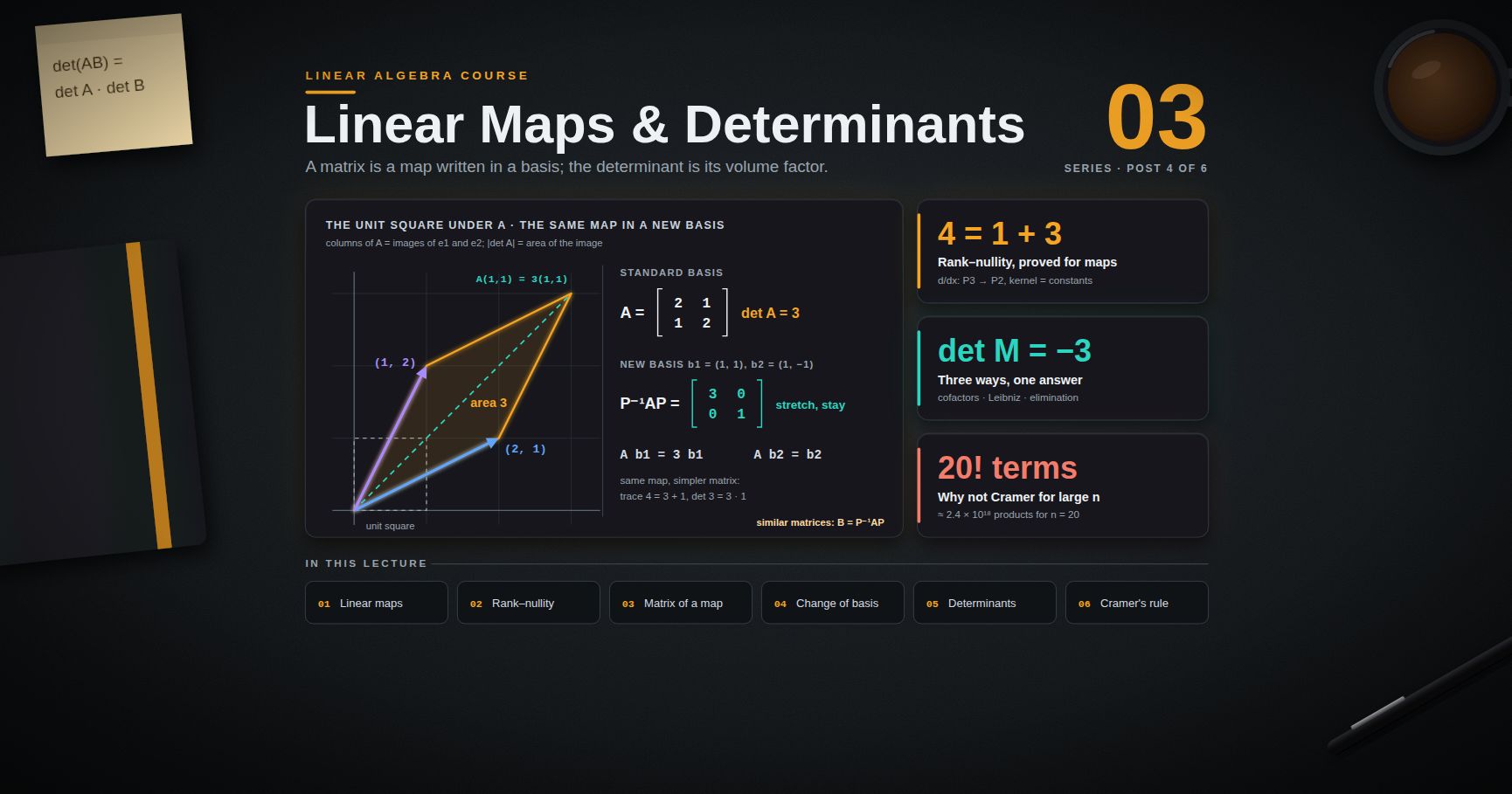
Linear Algebra — 01 · Matrix Algebra, Inverses and LU Factorization

In Linear Algebra 00 a matrix was only a compact way to write a system of equations. This post treats matrices as objects with their own algebra: they can be added, multiplied, transposed and — sometimes — inverted. Matrix multiplication is the operation that makes all of this interesting, so it gets four separate readings, each useful in a different situation. Then row operations become matrices themselves (elementary matrices), which turns Gaussian elimination into an algebraic statement: $A = LU$, a lower triangular matrix times an upper triangular one, or $PA = LU$ when rows must be exchanged. This factorization is how real software solves $A\mathbf{x} = \mathbf{b}$, and it explains a rule every numerical programmer learns early: do not compute $A^{-1}$ to solve a linear system.

Series map: 00 Vectors & Linear Systems → 01 Matrix Algebra, Inverses & LU (this post) → 02 Vector Spaces, Basis & Dimension → 03 Linear Maps, Change of Basis & Determinants → 04 Eigenvalues & Diagonalization → 05 Inner Products, Spectral Theorem & SVD.

---

Learning Outcome

• Multiply matrices in four ways — entry by entry, by columns, by rows, and as a sum of outer products — and know when each view is the helpful one.
• Explain why $AB \neq BA$ in general, and name other rules from ordinary algebra that fail for matrices.
• Use the transpose rules, including $(AB)^T = B^TA^T$, and recognise symmetric, triangular and permutation matrices.
• Multiply block (partitioned) matrices and do one step of block elimination.
• Write each row operation as an elementary matrix and invert it.
• Define the inverse, use the $2 \times 2$ formula, and compute $A^{-1}$ by Gauss–Jordan on $[\,A \mid I\,]$.
• State and prove the first version of the invertible matrix theorem.
• Factor $A = LU$ and $PA = LU$ by hand, prove that the LU factors are unique, and solve systems with two triangular solves.
• Count the cost of elimination (about $\tfrac23 n^3$ flops) and explain why solving with $A^{-1}$ is slower and less reliable.

---

Chapter 1 — Matrix operations

Terminology

• $m \times n$ matrix — a rectangular array of numbers with $m$ rows and $n$ columns. $a_{ij}$ is the entry in row $i$, column $j$.
• Square matrix — $m = n$. Its main diagonal is $a_{11}, a_{22}, \dots, a_{nn}$.
• Identity matrix $I_n$ — square, 1 on the main diagonal, 0 elsewhere. $I_n\mathbf{x} = \mathbf{x}$ for all $\mathbf{x}$.
• Zero matrix $0$ — all entries 0.
• Equal matrices — same size and the same entry in every position.

Addition and scalar multiplication work entry by entry, exactly as for vectors, and obey the same eight rules. Only matrices of the same size can be added.

The matrix product

If $A$ is $m \times n$ and $B$ is $n \times p$, the product $AB$ is the $m \times p$ matrix with entries

$$(AB)_{ij} = \sum_{k=1}^{n} a_{ik} b_{kj} = a_{i1}b_{1j} + a_{i2}b_{2j} + \dots + a_{in}b_{nj}.$$

The inner sizes must match: $(m \times n)(n \times p) = m \times p$. The example used throughout this chapter:

$$A = \begin{pmatrix} 1 & 2 \\ 3 & 4 \end{pmatrix}, \qquad B = \begin{pmatrix} 5 & 6 \\ 7 & 8 \end{pmatrix}, \qquad AB = \begin{pmatrix} 19 & 22 \\ 43 & 50 \end{pmatrix}.$$

Four ways to read AB

1. Entry by entry (row times column). $(AB)_{ij}$ is the dot product of row $i$ of $A$ with column $j$ of $B$. For example $(AB)_{12} = 1\cdot 6 + 2 \cdot 8 = 22$.

2. By columns. Column $j$ of $AB$ is $A$ times column $j$ of $B$:

$$AB = A\begin{pmatrix} \mathbf{b}_1 & \cdots & \mathbf{b}_p \end{pmatrix} = \begin{pmatrix} A\mathbf{b}_1 & \cdots & A\mathbf{b}_p \end{pmatrix}.$$

So every column of $AB$ is a combination of the columns of $A$. Here $A\mathbf{b}_1 = 5(1,3) + 7(2,4) = (19, 43)$.

3. By rows. Row $i$ of $AB$ is row $i$ of $A$ times $B$, so every row of $AB$ is a combination of the rows of $B$. Here row 1 is $1\cdot(5,6) + 2\cdot(7,8) = (19, 22)$. This is the view that explains elimination: row operations combine rows.

4. Columns times rows (sum of outer products). Multiply column $k$ of $A$ (an $m \times 1$ matrix) by row $k$ of $B$ (a $1 \times p$ matrix). Each such product is a full $m \times p$ matrix of rank at most one (Linear Algebra 02), and $AB$ is their sum:

$$AB = \sum_{k=1}^{n} \mathbf{a}_k \mathbf{b}^{*}_k = \begin{pmatrix} 1 \\ 3 \end{pmatrix}\begin{pmatrix} 5 & 6 \end{pmatrix} + \begin{pmatrix} 2 \\ 4 \end{pmatrix}\begin{pmatrix} 7 & 8 \end{pmatrix} = \begin{pmatrix} 5 & 6 \\ 15 & 18 \end{pmatrix} + \begin{pmatrix} 14 & 16 \\ 28 & 32 \end{pmatrix} = \begin{pmatrix} 19 & 22 \\ 43 & 50 \end{pmatrix}.$$

Here $\mathbf{b}^{*}_k$ denotes row $k$ of $B$. This view reappears in the SVD (Linear Algebra 05), which writes a matrix as a sum of rank-one pieces ordered by importance.

All four give the same numbers because each one computes $\sum_k a_{ik}b_{kj}$ in position $(i,j)$; they only group the work differently.

Trick: pick the view that matches the question. "Is $\mathbf{b}$ in the column space?" — columns. "What does a row operation do?" — rows. "What is the rank of $AB$?" — outer products. "Just give me a number" — entries.

Algebraic rules — and what fails

For matrices of compatible sizes:

• $A(BC) = (AB)C$ (associative), $A(B + C) = AB + AC$ and $(A + B)C = AC + BC$ (distributive), $c(AB) = (cA)B = A(cB)$, and $I_mA = A = AI_n$.

Proof of associativity. For a vector $\mathbf{x}$, $B\mathbf{x} = \sum_k x_k\mathbf{b}_k$, so $A(B\mathbf{x}) = \sum_k x_k A\mathbf{b}_k = (AB)\mathbf{x}$ by the column view. Apply this to each column $\mathbf{c}_j$ of $C$: column $j$ of $A(BC)$ is $A(B\mathbf{c}_j) = (AB)\mathbf{c}_j$, which is column $j$ of $(AB)C$. $\blacksquare$

Three rules from ordinary algebra fail:

1. Not commutative. $BA = \begin{pmatrix} 23 & 34 \\ 31 & 46 \end{pmatrix} \neq AB$. (Often only one of $AB$, $BA$ is even defined.)
2. Zero divisors. With $N = \begin{pmatrix} 0 & 1 \\ 0 & 0 \end{pmatrix}$, $N \neq 0$ but $N^2 = 0$.
3. No cancellation. $AB = AC$ does not imply $B = C$, even when $A \neq 0$ (take $A = N$, $B = N$, $C = 0$).

Common pitfall: $(A + B)^2 = A^2 + AB + BA + B^2$, not $A^2 + 2AB + B^2$. The two agree only when $AB = BA$.

---

Chapter 2 — Transpose and special matrices

Transpose

The transpose $A^T$ of an $m \times n$ matrix is the $n \times m$ matrix with $(A^T)_{ij} = a_{ji}$: rows become columns. Rules:

$$(A^T)^T = A, \qquad (A + B)^T = A^T + B^T, \qquad (cA)^T = cA^T, \qquad (AB)^T = B^TA^T.$$

Proof of the last rule. $((AB)^T)_{ij} = (AB)_{ji} = \sum_k a_{jk}b_{ki} = \sum_k (B^T)_{ik}(A^T)_{kj} = (B^TA^T)_{ij}$. $\blacksquare$

The order reverses, just like taking off shoes and socks. The dot product is a matrix product: $\mathbf{x}\cdot\mathbf{y} = \mathbf{x}^T\mathbf{y}$ (a $1 \times 1$ matrix).

Special matrices

Type	Definition	Useful facts
Diagonal	$a_{ij} = 0$ for $i \neq j$	products and powers act entry by entry on the diagonal
Upper triangular	$a_{ij} = 0$ for $i > j$	product of two upper triangular is upper triangular
Lower triangular	$a_{ij} = 0$ for $i < j$	same for lower; unit lower triangular has 1s on the diagonal
Symmetric	$A^T = A$	$A^TA$ and $AA^T$ are always symmetric
Permutation	the rows of $I$ in some order	$P\!A$ reorders the rows of $A$; $P^{-1} = P^T$

$A^TA$ is symmetric: $(A^TA)^T = A^T(A^T)^T = A^TA$. For example, with $X = \begin{pmatrix} 1 & 2 \\ 3 & 4 \\ 5 & 6 \end{pmatrix}$, $X^TX = \begin{pmatrix} 35 & 44 \\ 44 & 56 \end{pmatrix}$. This matrix is the heart of least squares (Linear Algebra 05).

Product of lower triangular matrices is lower triangular. If $a_{ik} = 0$ for $k > i$ and $b_{kj} = 0$ for $j > k$, then in $(AB)_{ij} = \sum_k a_{ik}b_{kj}$ a term can be nonzero only if $j \le k \le i$. When $i < j$ there is no such $k$, so $(AB)_{ij} = 0$. If both have unit diagonal, $(AB)_{ii} = a_{ii}b_{ii} = 1$. $\blacksquare$

Permutation matrices. Each row and each column of $P$ has exactly one 1. The rows of $P$ are orthonormal, so $PP^T = I$, which means $P^{-1} = P^T$.

---

Chapter 3 — Block matrices

A matrix can be cut by horizontal and vertical lines into blocks (submatrices). If the column cuts of $A$ match the row cuts of $B$, then $AB$ can be computed block by block, using the same formula as for numbers — but keeping the order of each product:

$$\begin{pmatrix} A_{11} & A_{12} \\ A_{21} & A_{22} \end{pmatrix} \begin{pmatrix} B_{11} & B_{12} \\ B_{21} & B_{22} \end{pmatrix} = \begin{pmatrix} A_{11}B_{11} + A_{12}B_{21} & A_{11}B_{12} + A_{12}B_{22} \\ A_{21}B_{11} + A_{22}B_{21} & A_{21}B_{12} + A_{22}B_{22} \end{pmatrix}.$$

The four views of Chapter 1 are all special cases: the column view cuts $B$ into columns, the row view cuts $A$ into rows, and the outer-product view cuts $A$ into columns and $B$ into rows.

Block elimination and the Schur complement

Let $M = \begin{pmatrix} A & B \\ C & D \end{pmatrix}$ with $A$ square and invertible. Eliminating the block $C$ is one block row operation — "block row 2 minus $CA^{-1}$ times block row 1":

$$\begin{pmatrix} I & 0 \\ -CA^{-1} & I \end{pmatrix} \begin{pmatrix} A & B \\ C & D \end{pmatrix} = \begin{pmatrix} A & B \\ 0 & D - CA^{-1}B \end{pmatrix}.$$

The block $S = D - CA^{-1}B$ is the Schur complement of $A$ in $M$. When every block is $1 \times 1$ this is exactly one step of ordinary elimination: $d - (c/a)b$. Schur complements appear in statistics (conditional covariance), in optimization and in domain-decomposition solvers.

Watch out: in block formulas every product must keep its order. $CA^{-1}B$ cannot be rewritten as $A^{-1}BC$ or $BCA^{-1}$.

---

Chapter 4 — Elementary matrices

An elementary matrix is the result of one row operation on the identity. Multiplying $A$ on the left by $E$ performs that row operation on $A$ (by the row view: row $i$ of $EA$ is row $i$ of $E$ times $A$).

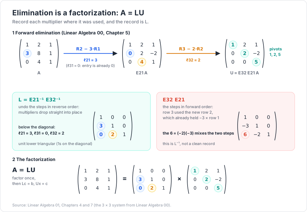
Using the $3 \times 3$ system from Linear Algebra 00,

$$A = \begin{pmatrix} 1 & 2 & 1 \\ 3 & 8 & 1 \\ 0 & 4 & 1 \end{pmatrix}, \qquad E_{21} = \begin{pmatrix} 1 & 0 & 0 \\ -3 & 1 & 0 \\ 0 & 0 & 1 \end{pmatrix}, \qquad E_{32} = \begin{pmatrix} 1 & 0 & 0 \\ 0 & 1 & 0 \\ 0 & -2 & 1 \end{pmatrix}.$$

$E_{21}$ subtracts 3 times row 1 from row 2; $E_{32}$ subtracts 2 times row 2 from row 3. (No $E_{31}$ is needed because $a_{31}$ is already 0.) Then

$$E_{32}E_{21}A = \begin{pmatrix} 1 & 2 & 1 \\ 0 & 2 & -2 \\ 0 & 0 & 5 \end{pmatrix} = U.$$

Every elementary matrix is invertible, and its inverse is elementary of the same type: undo "subtract $\ell$ times row $j$" by "add $\ell$ times row $j$"; undo a swap by the same swap; undo scaling by $c$ by scaling by $1/c$. For example

$$E_{21}^{-1} = \begin{pmatrix} 1 & 0 & 0 \\ 3 & 1 & 0 \\ 0 & 0 & 1 \end{pmatrix}.$$

The product in the "wrong" order is messy

$$E_{32}E_{21} = \begin{pmatrix} 1 & 0 & 0 \\ -3 & 1 & 0 \\ 6 & -2 & 1 \end{pmatrix}, \qquad E_{21}^{-1}E_{32}^{-1} = \begin{pmatrix} 1 & 0 & 0 \\ 3 & 1 & 0 \\ 0 & 2 & 1 \end{pmatrix}.$$

The entry 6 in the first product appears because row 3 is changed using the new row 2, which already contains $-3$ times row 1; indeed $6 = (-2)(-3)$. The inverses, multiplied in the opposite order, do not interact at all: the multipliers $3$ and $2$ simply drop into place. That clean matrix is $L$, and Chapter 7 is built on it. (The messy product $E_{32}E_{21}$ is $L^{-1}$.)

---

Chapter 5 — The inverse of a matrix

Definition and uniqueness

A square $n \times n$ matrix $A$ is invertible (or nonsingular) if there is a matrix $C$ with

$$CA = I \quad \text{and} \quad AC = I.$$

Then $C$ is called the inverse and written $A^{-1}$. A square matrix without an inverse is singular.

The inverse is unique. If $CA = I$ and $AD = I$, then $C = CI = C(AD) = (CA)D = ID = D$. $\blacksquare$ (This short argument even shows a left inverse and a right inverse must agree.)

Properties. If $A$ and $B$ are invertible $n \times n$ matrices, then

$$(A^{-1})^{-1} = A, \qquad (AB)^{-1} = B^{-1}A^{-1}, \qquad (A^T)^{-1} = (A^{-1})^T.$$

Proof. $(AB)(B^{-1}A^{-1}) = A(BB^{-1})A^{-1} = AA^{-1} = I$, and similarly in the other order. For the transpose, take the transpose of $AA^{-1} = I$: $(A^{-1})^TA^T = I$, and similarly $A^T(A^{-1})^T = I$. $\blacksquare$

If $A$ is invertible, $A\mathbf{x} = \mathbf{b}$ has exactly one solution for every $\mathbf{b}$, namely $\mathbf{x} = A^{-1}\mathbf{b}$: it is a solution because $A(A^{-1}\mathbf{b}) = \mathbf{b}$, and it is the only one because $A\mathbf{x} = \mathbf{b}$ implies $\mathbf{x} = A^{-1}A\mathbf{x} = A^{-1}\mathbf{b}$.

The 2 × 2 formula

$$\begin{pmatrix} a & b \\ c & d \end{pmatrix}^{-1} = \frac{1}{ad - bc}\begin{pmatrix} d & -b \\ -c & a \end{pmatrix}, \qquad \text{provided } ad - bc \neq 0.$$

Proof. Multiply: $\begin{pmatrix} a & b \\ c & d \end{pmatrix}\begin{pmatrix} d & -b \\ -c & a \end{pmatrix} = \begin{pmatrix} ad - bc & 0 \\ 0 & ad - bc \end{pmatrix}$, and the same holds in the other order. Divide by $ad - bc$. If $ad - bc = 0$, the same product shows $A$ times a matrix gives $0$; Exercise 6 shows $A$ is then singular. $\blacksquare$

The number $ad - bc$ is the determinant of the $2 \times 2$ matrix (Linear Algebra 03 defines it for all sizes). For $A = \begin{pmatrix} 1 & 2 \\ 3 & 4 \end{pmatrix}$: $ad - bc = 4 - 6 = -2$, so

$$A^{-1} = -\frac12 \begin{pmatrix} 4 & -2 \\ -3 & 1 \end{pmatrix} = \begin{pmatrix} -2 & 1 \\ 3/2 & -1/2 \end{pmatrix}.$$

Gauss–Jordan on [ A | I ]

Why it works. Suppose row operations $E_1, \dots, E_k$ turn $A$ into $I$: $E_k \cdots E_1 A = I$. Then $E_k\cdots E_1$ is a left inverse of $A$, and (by the invertible matrix theorem below) it is $A^{-1}$. Applying the same operations to $I$ produces $E_k \cdots E_1 I = A^{-1}$. So: row reduce the wide matrix $[\,A \mid I\,]$; if the left half becomes $I$, the right half is $A^{-1}$. If the left half develops a zero row, $A$ is singular.

Worked example. Take the "second difference" matrix

$$K = \begin{pmatrix} 2 & -1 & 0 \\ -1 & 2 & -1 \\ 0 & -1 & 2 \end{pmatrix}.$$

Forward elimination: $R_2 \leftarrow R_2 + \tfrac12 R_1$, then $R_3 \leftarrow R_3 + \tfrac23 R_2$:

$$\left(\begin{array}{ccc|ccc} 2 & -1 & 0 & 1 & 0 & 0 \\ 0 & 3/2 & -1 & 1/2 & 1 & 0 \\ 0 & 0 & 4/3 & 1/3 & 2/3 & 1 \end{array}\right).$$

The pivots are $2, \tfrac32, \tfrac43$. Backward elimination: $R_2 \leftarrow R_2 + \tfrac34 R_3$, then $R_1 \leftarrow R_1 + \tfrac23 R_2$:

$$\left(\begin{array}{ccc|ccc} 2 & 0 & 0 & 3/2 & 1 & 1/2 \\ 0 & 3/2 & 0 & 3/4 & 3/2 & 3/4 \\ 0 & 0 & 4/3 & 1/3 & 2/3 & 1 \end{array}\right).$$

Divide each row by its pivot:

$$K^{-1} = \begin{pmatrix} 3/4 & 1/2 & 1/4 \\ 1/2 & 1 & 1/2 \\ 1/4 & 1/2 & 3/4 \end{pmatrix} = \frac14\begin{pmatrix} 3 & 2 & 1 \\ 2 & 4 & 2 \\ 1 & 2 & 3 \end{pmatrix}.$$

Two observations that matter later. $K$ is symmetric and so is $K^{-1}$ (Exercise 7). And $K$ is tridiagonal — mostly zeros — but $K^{-1}$ is completely full. Keep that in mind for Chapter 8.

---

Chapter 6 — The invertible matrix theorem

Theorem. For a square $n \times n$ matrix $A$, the following are equivalent (all true or all false):

1. $A$ is invertible.
2. $A$ is row equivalent to $I_n$.
3. $A$ has $n$ pivot positions.
4. $A\mathbf{x} = \mathbf{0}$ has only the trivial solution.
5. The columns of $A$ are linearly independent.
6. $A\mathbf{x} = \mathbf{b}$ has at least one solution for every $\mathbf{b} \in \mathbb{R}^n$.
7. The columns of $A$ span $\mathbb{R}^n$.
8. There is an $n \times n$ matrix $C$ with $CA = I$.
9. There is an $n \times n$ matrix $D$ with $AD = I$.
10. $A^T$ is invertible.
11. $A$ is a product of elementary matrices.

Proof. (1) ⇒ (8) and (1) ⇒ (9): take $C = D = A^{-1}$.

(8) ⇒ (4): if $A\mathbf{x} = \mathbf{0}$ then $\mathbf{x} = CA\mathbf{x} = C\mathbf{0} = \mathbf{0}$.

(4) ⇔ (5): this is the definition of independence (Linear Algebra 00, Chapter 8).

(4) ⇒ (3): only the trivial solution means no free variables, so every one of the $n$ columns is a pivot column.

(3) ⇒ (2): $n$ pivots in an $n \times n$ matrix means one pivot in every row and every column, on the diagonal, so the RREF is $I_n$.

(2) ⇒ (11): $E_k\cdots E_1A = I$ gives $A = E_1^{-1}\cdots E_k^{-1}$, a product of elementary matrices.

(11) ⇒ (1): elementary matrices are invertible, and so is any product of invertible matrices.

(9) ⇒ (6): given $\mathbf{b}$, the vector $\mathbf{x} = D\mathbf{b}$ satisfies $A\mathbf{x} = AD\mathbf{b} = \mathbf{b}$.

(6) ⇔ (7): $A\mathbf{x}$ ranges over all combinations of the columns (Linear Algebra 00).

(6) ⇒ (3): if $A$ had fewer than $n$ pivots, its echelon form $U$ would have a zero last row. Choose $\mathbf{c}$ with last entry 1; then $U\mathbf{x} = \mathbf{c}$ is inconsistent, and undoing the row operations on $\mathbf{c}$ gives a $\mathbf{b}$ with $A\mathbf{x} = \mathbf{b}$ inconsistent, contradicting (6).

(1) ⇔ (10): if $A$ is invertible, $(A^{-1})^T$ inverts $A^T$ (Chapter 5); apply this to $A^T$ for the converse.

Every statement is now linked to every other. $\blacksquare$

Corollary (one-sided is enough). If $A$ and $B$ are square and $AB = I$, then $BA = I$ and $B = A^{-1}$. Proof: $AB = I$ is statement (9) for $A$, so $A$ is invertible; multiply $AB = I$ on the left by $A^{-1}$ to get $B = A^{-1}$. $\blacksquare$

Watch out: the corollary needs square matrices. For $A = \begin{pmatrix} 1 & 0 \end{pmatrix}$ and $B = \begin{pmatrix} 1 \\ 0 \end{pmatrix}$, $AB = (1) = I_1$ but $BA = \begin{pmatrix} 1 & 0 \\ 0 & 0 \end{pmatrix} \neq I_2$.

Linear Algebra 02, 03 and 04 add more lines to this list: rank $n$, null space $\{\mathbf{0}\}$, $\det A \neq 0$, and $0$ is not an eigenvalue.

---

Chapter 7 — LU factorization

From elimination to A = LU

Suppose elimination on $A$ needs no row exchanges. Then only replacement operations "row $i$ minus $\ell_{ij}$ times row $j$" (with $i > j$) are used, and

$$(E_{32}E_{31}E_{21})\,A = U \qquad\Longrightarrow\qquad A = (E_{21}^{-1}E_{31}^{-1}E_{32}^{-1})\,U = LU$$

(written for $n = 3$; larger $n$ is the same). $U$ is upper triangular with the pivots on its diagonal. $L$ is unit lower triangular, and as Chapter 4 showed, its entries below the diagonal are exactly the multipliers: $L_{ij} = \ell_{ij}$.

For the running example, the multipliers were $\ell_{21} = 3$, $\ell_{31} = 0$, $\ell_{32} = 2$, so

$$\begin{pmatrix} 1 & 2 & 1 \\ 3 & 8 & 1 \\ 0 & 4 & 1 \end{pmatrix} = \begin{pmatrix} 1 & 0 & 0 \\ 3 & 1 & 0 \\ 0 & 2 & 1 \end{pmatrix} \begin{pmatrix} 1 & 2 & 1 \\ 0 & 2 & -2 \\ 0 & 0 & 5 \end{pmatrix}.$$

Multiply it out to check: row 2 of $LU$ is $3(1,2,1) + (0,2,-2) = (3, 8, 1)$, and row 3 is $2(0,2,-2) + (0,0,5) = (0, 4, 1)$.

Solving with L and U

$A\mathbf{x} = \mathbf{b}$ becomes $L(U\mathbf{x}) = \mathbf{b}$. Put $\mathbf{c} = U\mathbf{x}$ and solve two triangular systems:

1. Forward substitution $L\mathbf{c} = \mathbf{b}$ (top to bottom).
2. Back substitution $U\mathbf{x} = \mathbf{c}$ (bottom to top).

With $\mathbf{b} = (2, 12, 2)$: $c_1 = 2$; $3c_1 + c_2 = 12$ gives $c_2 = 6$; $2c_2 + c_3 = 2$ gives $c_3 = -10$. So $\mathbf{c} = (2, 6, -10)$ — exactly the right-hand side that elimination produced in Linear Algebra 00. Then $U\mathbf{x} = \mathbf{c}$ gives $z = -2$, $y = 1$, $x = 2$, as before.

The point: the factorization is done once; each new right-hand side then costs only two cheap triangular solves.

LDU and the symmetric case

Divide each row of $U$ by its pivot to get $A = LDU'$ with $D$ the diagonal matrix of pivots and $U'$ unit upper triangular. For the example, $D = \operatorname{diag}(1, 2, 5)$ and

$$U' = \begin{pmatrix} 1 & 2 & 1 \\ 0 & 1 & -1 \\ 0 & 0 & 1 \end{pmatrix}.$$

When $A$ is symmetric and has an LU factorization, $U' = L^T$, so $A = LDL^T$. For a symmetric matrix with all pivots positive this becomes the Cholesky factorization $A = (LD^{1/2})(LD^{1/2})^T$, which costs about half as much as LU.

Uniqueness

Theorem. If $A$ is invertible and $A = L_1U_1 = L_2U_2$ with $L_1, L_2$ unit lower triangular and $U_1, U_2$ upper triangular, then $L_1 = L_2$ and $U_1 = U_2$.

Proof. Since $A$ is invertible, so are the $U_i$ (and the unit-diagonal $L_i$ always are). From $L_1U_1 = L_2U_2$,

$$L_2^{-1}L_1 = U_2U_1^{-1}.$$

The left side is unit lower triangular (inverses and products of unit lower triangular matrices are unit lower triangular — Chapter 2 and Exercise 5), and the right side is upper triangular. A matrix that is both is diagonal, and its diagonal is all 1s from the left side. So both sides equal $I$, which gives $L_1 = L_2$ and $U_1 = U_2$. $\blacksquare$

Row exchanges: PA = LU

Elimination breaks down when a zero appears in a pivot position. Example:

$$A = \begin{pmatrix} 0 & 1 & 1 \\ 1 & 2 & 1 \\ 2 & 7 & 9 \end{pmatrix}.$$

The (1,1) entry is 0, so swap rows 1 and 2 first. If all the exchanges are done at the start, they form one permutation matrix $P$, and $PA$ factors without further trouble:

$$P = \begin{pmatrix} 0 & 1 & 0 \\ 1 & 0 & 0 \\ 0 & 0 & 1 \end{pmatrix}, \qquad PA = \begin{pmatrix} 1 & 2 & 1 \\ 0 & 1 & 1 \\ 2 & 7 & 9 \end{pmatrix} = \begin{pmatrix} 1 & 0 & 0 \\ 0 & 1 & 0 \\ 2 & 3 & 1 \end{pmatrix} \begin{pmatrix} 1 & 2 & 1 \\ 0 & 1 & 1 \\ 0 & 0 & 4 \end{pmatrix}.$$

The multipliers were $\ell_{21} = 0$, $\ell_{31} = 2$ (row 3 becomes $(0, 3, 7)$), then $\ell_{32} = 3$ (row 3 becomes $(0, 0, 4)$).

Theorem. For every invertible $A$ there is a permutation matrix $P$ such that $PA = LU$ with $L$ unit lower triangular and $U$ upper triangular with nonzero pivots. An invertible $A$ has an LU factorization with no exchanges ($P = I$) exactly when every leading principal submatrix (the top-left $k \times k$ block, $k = 1, \dots, n$) is invertible.

To solve $A\mathbf{x} = \mathbf{b}$ from $PA = LU$: $LU\mathbf{x} = P\mathbf{b}$, so permute $\mathbf{b}$, then do the two triangular solves.

Common pitfall: after factoring $PA = LU$, forgetting to apply $P$ to $\mathbf{b}$. The factorization is of $PA$, not of $A$.

---

Chapter 8 — Cost, and why not to compute the inverse

Counting flops

A flop is one floating-point add, subtract, multiply or divide. At elimination step $k$ of an $n \times n$ matrix, each of the $n - k$ rows below the pivot needs one division (its multiplier) and a multiply and a subtract for each of the remaining $n - k$ entries. So step $k$ costs $(n - k)\bigl(2(n - k) + 1\bigr)$ flops, and in total

$$\sum_{k=1}^{n} \bigl( 2(n-k)^2 + (n-k) \bigr) = \frac{2}{3}n^3 - \frac12 n^2 - \frac16 n \approx \frac23 n^3.$$

Each triangular solve costs about $n^2$ flops. So for $n = 1000$: roughly $6.7 \times 10^8$ flops to factor, then only about $2 \times 10^6$ per right-hand side.

Why solving with the inverse is the wrong way

1. Speed. Forming $A^{-1}$ costs about $2n^3$ flops — roughly three times the LU factorization — and then $A^{-1}\mathbf{b}$ still costs $2n^2$, the same as the two triangular solves it was supposed to replace. There is nothing to gain even with many right-hand sides, because LU is reusable too.
2. Accuracy. Gaussian elimination with partial pivoting is backward stable in practice: the computed $\mathbf{x}$ exactly solves a system with a very slightly perturbed $A$. Multiplying by a computed inverse does not have this guarantee in general, and its residual $\lVert \mathbf{b} - A\mathbf{x} \rVert$ is typically larger (Higham, Chapters 9 and 14).
3. Structure. A banded or sparse matrix has banded or sparse LU factors (without pivoting, a tridiagonal $K$ has bidiagonal $L$ and $U$), but its inverse is usually full — as $K^{-1}$ in Chapter 5 showed. For large sparse problems the inverse may not even fit in memory.

In code this means numpy.linalg.solve(A, b) (which calls LAPACK's LU-based gesv), or scipy.linalg.lu_factor once and lu_solve for each right-hand side — never inv(A) @ b.

Trick: read $A^{-1}\mathbf{b}$ in a formula as "the solution of $A\mathbf{x} = \mathbf{b}$", not as an instruction to invert. The same holds for expressions like $A^{-1}B$ (solve with many right-hand sides) and $\mathbf{c}^TA^{-1}\mathbf{b}$ (one solve, then one dot product).

---

Practice Exercises

Exercise 1 — Order matters

Let $A = \begin{pmatrix} 1 & 0 \\ 2 & 1 \end{pmatrix}$ and $B = \begin{pmatrix} 3 & 1 \\ 0 & 2 \end{pmatrix}$. Compute $AB$ and $BA$. Describe $AB$ with the row view.

Solution

$AB = \begin{pmatrix} 3 & 1 \\ 6 & 4 \end{pmatrix}$ and $BA = \begin{pmatrix} 5 & 1 \\ 4 & 2 \end{pmatrix}$, which differ. Row view: $A$ is an elementary matrix ("add 2 times row 1 to row 2"), so $AB$ is $B$ with row 2 replaced by $(0,2) + 2(3,1) = (6, 4)$.

Exercise 2 — Transpose of a triple product

Prove $(ABC)^T = C^TB^TA^T$, and deduce that $B^TAB$ is symmetric whenever $A$ is symmetric.

Solution

$(ABC)^T = ((AB)C)^T = C^T(AB)^T = C^TB^TA^T$. If $A^T = A$, then $(B^TAB)^T = B^TA^T(B^T)^T = B^TAB$.

Exercise 3 — Inverses

Find the inverse of $\begin{pmatrix} 2 & 5 \\ 1 & 3 \end{pmatrix}$ with the $2 \times 2$ formula, and of $\begin{pmatrix} 1 & 2 & 3 \\ 0 & 1 & 4 \\ 5 & 6 & 0 \end{pmatrix}$ by Gauss–Jordan.

Solution

$ad - bc = 6 - 5 = 1$, so the first inverse is $\begin{pmatrix} 3 & -5 \\ -1 & 2 \end{pmatrix}$.

For the $3 \times 3$ matrix, row reducing $[\,A \mid I\,]$ gives

$$A^{-1} = \begin{pmatrix} -24 & 18 & 5 \\ 20 & -15 & -4 \\ -5 & 4 & 1 \end{pmatrix}.$$

Check one entry of $AA^{-1}$: row 3 of $A$ times column 1 of $A^{-1}$ is $5(-24) + 6(20) + 0 = 0$, as it should be.

Exercise 4 — LU by hand

Factor $A = \begin{pmatrix} 2 & 1 & 1 \\ 4 & -6 & 0 \\ -2 & 7 & 2 \end{pmatrix}$ as $LU$.

Solution

$\ell_{21} = 4/2 = 2$ and $\ell_{31} = -2/2 = -1$ give rows $(0, -8, -2)$ and $(0, 8, 3)$. Then $\ell_{32} = 8/(-8) = -1$ gives row 3 $= (0, 0, 1)$. So

$$L = \begin{pmatrix} 1 & 0 & 0 \\ 2 & 1 & 0 \\ -1 & -1 & 1 \end{pmatrix}, \qquad U = \begin{pmatrix} 2 & 1 & 1 \\ 0 & -8 & -2 \\ 0 & 0 & 1 \end{pmatrix}.$$

Pivots $2, -8, 1$.

Exercise 5 — Inverse of a unit lower triangular matrix

Show that the inverse of a unit lower triangular matrix is unit lower triangular (this completes the uniqueness proof in Chapter 7).

Solution

A unit lower triangular $L$ reduces to $I$ using only operations "row $i$ minus a multiple of row $j$" with $i > j$ (no swaps, no scaling, since the pivots are already 1). Each such elementary matrix is unit lower triangular, so $L^{-1}$, the product of these elementary matrices, is unit lower triangular by the Chapter 2 result.

Exercise 6 — A zero pivot that cannot be fixed

Show that if $ad - bc = 0$ then $A = \begin{pmatrix} a & b \\ c & d \end{pmatrix}$ is singular. Also show that $\begin{pmatrix} 0 & 1 \\ 1 & 1 \end{pmatrix}$ is invertible but has no LU factorization without a row exchange.

Solution

If $A = 0$ it is singular. Otherwise $M = \begin{pmatrix} d & -b \\ -c & a \end{pmatrix} \neq 0$ and $AM = 0$. If $A$ were invertible, $M = A^{-1}AM = 0$, a contradiction.

For the second matrix, $ad - bc = -1 \neq 0$, so it is invertible. If $\begin{pmatrix} 0 & 1 \\ 1 & 1 \end{pmatrix} = \begin{pmatrix} 1 & 0 \\ \ell & 1 \end{pmatrix}\begin{pmatrix} u_{11} & u_{12} \\ 0 & u_{22} \end{pmatrix}$, the (1,1) entry forces $u_{11} = 0$, but then the (2,1) entry is $\ell u_{11} = 0 \neq 1$. Its first leading principal submatrix $(0)$ is singular, as the theorem predicts. With the swap, $PA = \begin{pmatrix} 1 & 1 \\ 0 & 1 \end{pmatrix} = I \cdot U$.

Exercise 7 — Symmetric inverse

Prove: if $A$ is symmetric and invertible, then $A^{-1}$ is symmetric.

Solution

$(A^{-1})^T = (A^T)^{-1} = A^{-1}$, using the transpose rule for inverses from Chapter 5 and $A^T = A$.

---

Cheat-sheet

Topic	Key fact
Product size	$(m \times n)(n \times p) = m \times p$
Four views of $AB$	entries, columns $A\mathbf{b}_j$, rows, sum of outer products
Fails for matrices	$AB = BA$, cancellation, "no zero divisors"
Transpose	$(AB)^T = B^TA^T$; $A^TA$ is symmetric
Block product	same formula as scalars, order kept
Schur complement	$D - CA^{-1}B$
Elementary matrix	row operation on $I$; multiply on the left
$2 \times 2$ inverse	swap $a, d$; negate $b, c$; divide by $ad - bc \neq 0$
Inverse rules	$(AB)^{-1} = B^{-1}A^{-1}$, $(A^T)^{-1} = (A^{-1})^T$
Compute $A^{-1}$	Gauss–Jordan on $[\,A \mid I\,]$
Square, $AB = I$	then $BA = I$
$A = LU$	$L$ unit lower with multipliers; $U$ upper with pivots
Row exchanges	$PA = LU$; solve $LU\mathbf{x} = P\mathbf{b}$
LU cost	$\approx \tfrac23 n^3$ flops; each triangular solve $\approx n^2$
Solve, do not invert	solve(A, b) or lu_factor + lu_solve

---

What's next

Linear Algebra 02 steps back from matrices to the structures they act on. It defines a vector space by axioms (so polynomials, functions and matrices count), then subspaces, span, independence, basis and dimension — with a full proof that dimension is well defined (the Steinitz exchange lemma). It then studies the four fundamental subspaces of a matrix, proves that row rank equals column rank, and proves rank–nullity in matrix form.

---

References

• Gilbert Strang, Introduction to Linear Algebra, 6th edition, Wellesley-Cambridge Press, 2023 — Chapter 2 (elimination matrices, inverses, $A = LU$, transposes and permutations).
• David C. Lay, Steven R. Lay and Judi J. McDonald, Linear Algebra and Its Applications, 6th edition, Pearson, 2021 — Chapter 2 (matrix operations, the invertible matrix theorem, partitioned matrices, LU).
• Lloyd N. Trefethen and David Bau III, Numerical Linear Algebra, SIAM, 1997 — Lectures 20–21 (Gaussian elimination, operation count, pivoting).
• Gene H. Golub and Charles F. Van Loan, Matrix Computations, 4th edition, Johns Hopkins University Press, 2013 — Chapter 3 (LU and its variants).
• Nicholas J. Higham, Accuracy and Stability of Numerical Algorithms, 2nd edition, SIAM, 2002 — Chapter 9 (LU factorization and linear equations) and Chapter 14 (matrix inversion).
• MIT OpenCourseWare, 18.06 Linear Algebra, Spring 2010 (Gilbert Strang) — Lectures 3–5: multiplication and inverses, $A = LU$, transposes and permutations.

Note: this post is in progress. Planned additions: a proof of the leading-principal-submatrix condition for LU without exchanges, a worked partial-pivoting example in three-digit arithmetic, and a short numerical demo comparing solve with inv(A) @ b on an ill-conditioned matrix.