Linear Algebra — 04 · Eigenvalues, Eigenvectors and Diagonalization

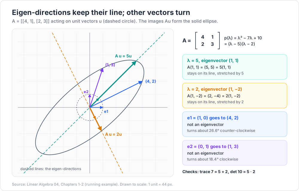
Most vectors change direction when a matrix acts on them. A few special directions do not: the matrix only stretches, shrinks or flips them. Those directions are the eigenvectors, and the stretch factors are the eigenvalues. If a matrix has enough eigenvectors to form a basis, then in that basis it is diagonal — every hard question about the matrix (its powers, its long-run behaviour, the differential equation it drives) splits into $n$ independent one-dimensional questions. This post builds the theory with proofs, then uses it on Fibonacci numbers, a Markov chain, a system of differential equations, and the power-iteration algorithm. It relies on the determinant and on change of basis from Linear Algebra 03.

Series map: 00 Vectors & Linear Systems → 01 Matrix Algebra, Inverses & LU → 02 Vector Spaces, Basis & Dimension → 03 Linear Maps, Change of Basis & Determinants → 04 Eigenvalues & Diagonalization (this post) → 05 Inner Products, Spectral Theorem & SVD.

---

Learning Outcome

• Define eigenvalues, eigenvectors and eigenspaces, and describe them geometrically for common maps of the plane.
• Find eigenvalues from the characteristic polynomial and eigenvectors from null spaces, for $2 \times 2$ and $3 \times 3$ matrices.
• Distinguish algebraic from geometric multiplicity, and prove that eigenvectors for distinct eigenvalues are independent.
• Decide whether a matrix is diagonalizable, and write $A = PDP^{-1}$ when it is.
• Compute $A^k$ and solve difference equations (Fibonacci, Markov chains) by diagonalization.
• Handle complex eigenvalues, and use trace = sum and determinant = product of the eigenvalues as checks.
• State and use the Cayley–Hamilton theorem; recognise a defective matrix and state the Jordan form.
• Solve $x' = Ax$ with $e^{At} = Pe^{Dt}P^{-1}$, and explain how power iteration finds the dominant eigenvalue.

---

Chapter 1 — Eigenvalues and eigenvectors

Terminology

• Eigenvector of a square matrix $A$ (or a linear operator $T: V \to V$) — a nonzero vector $v$ with $Av = \lambda v$ for some scalar $\lambda$.
• Eigenvalue — a scalar $\lambda$ for which such a nonzero $v$ exists. "Eigen" is German for "own" or "characteristic".
• Eigenspace $E_\lambda = \{v : Av = \lambda v\} = N(A - \lambda I)$ — all eigenvectors for $\lambda$, together with $0$. It is a subspace.
• Spectrum — the set of all eigenvalues of $A$.
• Diagonalizable — similar to a diagonal matrix: $A = PDP^{-1}$ with $D$ diagonal and $P$ invertible.

The zero vector is excluded as an eigenvector because $A0 = \lambda 0$ holds for every $\lambda$ and would say nothing. The eigenvalue $\lambda = 0$, on the other hand, is allowed: $Av = 0v$ with $v \neq 0$ means $v$ is in the null space, so $0$ is an eigenvalue exactly when $A$ is singular.

What it means geometrically

$Av = \lambda v$ says: the line through $v$ is mapped into itself. Along that line, $A$ acts as multiplication by the number $\lambda$. If $\lambda > 1$ the line is stretched, $0 < \lambda < 1$ shrinks it, $\lambda < 0$ flips it, $\lambda = 0$ collapses it to the origin.

The maps of the plane from Linear Algebra 03:

Map	Eigenvalues and eigen-directions
Projection onto a line $L$	$1$ on $L$ (kept), $0$ on the perpendicular line (killed)
Reflection in a line $L$	$1$ on $L$, $-1$ on the perpendicular line
Rotation by $\theta$, $0 < \theta < 180°$	no real eigenvector — every direction turns; complex eigenvalues $e^{\pm i\theta}$ (Chapter 6)
Shear $\begin{pmatrix} 1 & k \\ 0 & 1\end{pmatrix}$, $k \neq 0$	only $1$, only along the $x$-axis — not enough eigenvectors (Chapter 4)
Scaling $\operatorname{diag}(a, b)$	$a$ along $e_1$, $b$ along $e_2$

Running example. Throughout the post,

$$A = \begin{pmatrix} 4 & 1 \\ 2 & 3 \end{pmatrix}.$$

Check two directions: $A(1, 1) = (5, 5) = 5(1, 1)$ and $A(1, -2) = (2, -4) = 2(1, -2)$. So $(1,1)$ is an eigenvector with eigenvalue 5 and $(1, -2)$ is one with eigenvalue 2. A vector off these lines turns: $e_1 = (1,0)$ goes to $(4, 2)$, a turn of about $26.6°$ counter-clockwise, and $e_2 = (0,1)$ goes to $(1, 3)$, a turn of about $18.4°$ clockwise.

---

Chapter 2 — The characteristic polynomial

From a nonlinear problem to a determinant

$Av = \lambda v$ has two unknowns multiplied together ($\lambda$ and $v$), so it is not a linear system. Rewrite it as

$$(A - \lambda I)v = 0, \qquad v \neq 0.$$

A nonzero solution exists exactly when $A - \lambda I$ is singular, which by Linear Algebra 03 happens exactly when its determinant is zero. So:

Theorem 1. $\lambda$ is an eigenvalue of $A$ if and only if $\det(\lambda I - A) = 0$.

The function $p_A(\lambda) = \det(\lambda I - A)$ is the characteristic polynomial of $A$. Expanding the determinant with the Leibniz formula shows it is a polynomial of degree $n$ with leading coefficient 1. (Some books use $\det(A - \lambda I) = (-1)^n p_A(\lambda)$; the roots are the same.)

The recipe is therefore two steps: (1) find the roots of $p_A$; (2) for each root $\lambda$, find the null space of $A - \lambda I$ by elimination.

The shortcut for 2 × 2 matrices

For $A = \begin{pmatrix} a & b \\ c & d\end{pmatrix}$,

$$p_A(\lambda) = (\lambda - a)(\lambda - d) - bc = \lambda^2 - (a + d)\lambda + (ad - bc) = \lambda^2 - (\operatorname{tr}A)\,\lambda + \det A.$$

Worked example. For the running example, $\operatorname{tr}A = 7$ and $\det A = 12 - 2 = 10$:

$$p_A(\lambda) = \lambda^2 - 7\lambda + 10 = (\lambda - 5)(\lambda - 2).$$

For $\lambda = 5$: $A - 5I = \begin{pmatrix} -1 & 1 \\ 2 & -2\end{pmatrix}$, whose null space is spanned by $(1, 1)$. For $\lambda = 2$: $A - 2I = \begin{pmatrix} 2 & 1 \\ 2 & 1\end{pmatrix}$, null space spanned by $(1, -2)$. This matches Chapter 1.

Trick: After finding a $2 \times 2$ matrix $A - \lambda I$, you do not need to row-reduce. If the first row is $(p, q)$, then $(q, -p)$ (or $(-q, p)$) is in the null space. The second row must be a multiple of the first — if it is not, $\lambda$ was computed wrongly.

A 3 × 3 example with a repeated eigenvalue

$$B = \begin{pmatrix} 2 & 1 & 1 \\ 1 & 2 & 1 \\ 1 & 1 & 2 \end{pmatrix}, \qquad p_B(\lambda) = \lambda^3 - 6\lambda^2 + 9\lambda - 4 = (\lambda - 4)(\lambda - 1)^2.$$

(A quick way to see this: $B = I + J$ where $J$ is the all-ones matrix. $J$ has rank 1, so $0$ is an eigenvalue of $J$ with a two-dimensional eigenspace, and $J(1,1,1) = 3(1,1,1)$. Adding $I$ adds 1 to every eigenvalue.)

• $\lambda = 4$: $B - 4I$ has null space spanned by $(1, 1, 1)$.
• $\lambda = 1$: $B - I = J$, every row is $(1, 1, 1)$, so the null space is the plane $x + y + z = 0$, spanned by $(-1, 1, 0)$ and $(-1, 0, 1)$.

The eigenvalue 1 is a double root and has a two-dimensional eigenspace. That is the good case, as Chapter 3 explains.

Easy cases and invariance

• Triangular matrices: $\lambda I - A$ is triangular, so $p_A(\lambda) = \prod (\lambda - a_{ii})$. The eigenvalues are the diagonal entries.
• Similar matrices have the same characteristic polynomial. If $B = P^{-1}AP$ then $\lambda I - B = P^{-1}(\lambda I - A)P$, so by the product rule $\det(\lambda I - B) = \det(\lambda I - A)$. So eigenvalues belong to the operator, not to a particular matrix of it (Linear Algebra 03, similarity invariants).
• $A$ and $A^T$ have the same characteristic polynomial (because $\det M^T = \det M$), but usually different eigenvectors.

Common pitfall: Row operations change eigenvalues. Row-reducing $A$ first and then reading off the diagonal gives the pivots, not the eigenvalues. Row-reduce $A - \lambda I$ (to find eigenvectors), never $A$.

Trace and determinant from the eigenvalues

Over $\mathbb{C}$, every polynomial factors completely (fundamental theorem of algebra), so $p_A(\lambda) = (\lambda - \lambda_1)\cdots(\lambda - \lambda_n)$, with eigenvalues repeated by multiplicity.

Theorem 2. $\operatorname{tr} A = \lambda_1 + \dots + \lambda_n$ and $\det A = \lambda_1 \lambda_2 \cdots \lambda_n$.

Proof. Put $\lambda = 0$ in $\det(\lambda I - A) = \prod(\lambda - \lambda_i)$: $\det(-A) = \prod(-\lambda_i)$, that is $(-1)^n \det A = (-1)^n \prod \lambda_i$. For the trace, compare the coefficients of $\lambda^{n-1}$. On the right it is $-\sum \lambda_i$. On the left, in the Leibniz expansion of $\det(\lambda I - A)$, any term other than the diagonal product uses at most $n - 2$ diagonal entries, so has degree at most $n - 2$ in $\lambda$. The diagonal product $\prod(\lambda - a_{ii})$ contributes $-\sum a_{ii} = -\operatorname{tr}A$. ∎

Checks: for $A$, $5 + 2 = 7 = \operatorname{tr}A$ and $5 \cdot 2 = 10 = \det A$. For $B$, $4 + 1 + 1 = 6$ and $4 \cdot 1 \cdot 1 = 4 = \det B$.

---

Chapter 3 — Multiplicities and independence

Two kinds of multiplicity

For an eigenvalue $\lambda_0$:

• Algebraic multiplicity — how many times $\lambda_0$ is a root of $p_A$ (the power of $(\lambda - \lambda_0)$ in the factorisation).
• Geometric multiplicity — $\dim E_{\lambda_0} = \dim N(A - \lambda_0 I)$, the number of independent eigenvectors for $\lambda_0$.

Theorem 3. $1 \le \text{geometric multiplicity} \le \text{algebraic multiplicity}$.

Proof. The lower bound holds because an eigenvalue has at least one eigenvector. For the upper bound let $g = \dim E_{\lambda_0}$ with basis $v_1, \dots, v_g$, and extend it to a basis $v_1, \dots, v_n$ of $\mathbb{R}^n$. With $P = (v_1 \cdots v_n)$, the first $g$ columns of $P^{-1}AP$ are $\lambda_0 e_1, \dots, \lambda_0 e_g$, so

$$P^{-1}AP = \begin{pmatrix} \lambda_0 I_g & X \\ 0 & Y \end{pmatrix}.$$

Similar matrices share the characteristic polynomial, and the block triangular determinant rule gives $p_A(\lambda) = (\lambda - \lambda_0)^g \det(\lambda I - Y)$. So $(\lambda - \lambda_0)^g$ divides $p_A$, and the algebraic multiplicity is at least $g$. ∎

In the example $B$, the eigenvalue 1 has algebraic multiplicity 2 and geometric multiplicity 2. For the shear $\begin{pmatrix} 1 & 1 \\ 0 & 1\end{pmatrix}$, the eigenvalue 1 has algebraic multiplicity 2 but geometric multiplicity 1. That gap is exactly what stops a matrix from being diagonalizable.

Eigenvectors for different eigenvalues are independent

Theorem 4. If $v_1, \dots, v_k$ are eigenvectors of $A$ for distinct eigenvalues $\lambda_1, \dots, \lambda_k$, then $v_1, \dots, v_k$ are linearly independent.

Proof. Suppose not. Let $m$ be the smallest index such that $v_m$ is a combination of $v_1, \dots, v_{m-1}$; then $v_1, \dots, v_{m-1}$ are independent, and $m \ge 2$ since $v_1 \neq 0$. Write

$$v_m = c_1 v_1 + \dots + c_{m-1} v_{m-1}.$$

Apply $A$: $\lambda_m v_m = c_1 \lambda_1 v_1 + \dots + c_{m-1}\lambda_{m-1} v_{m-1}$. Subtract $\lambda_m$ times the first equation:

$$0 = c_1(\lambda_1 - \lambda_m) v_1 + \dots + c_{m-1}(\lambda_{m-1} - \lambda_m) v_{m-1}.$$

By independence each $c_i(\lambda_i - \lambda_m) = 0$, and since the eigenvalues are distinct, each $c_i = 0$. Then $v_m = 0$, which is impossible for an eigenvector. ∎

The same argument shows more: if you take a basis of each eigenspace and put them together, the combined list is still independent. So the sum of the geometric multiplicities is the number of independent eigenvectors the matrix has in total.

Corollary 5. An $n \times n$ matrix with $n$ distinct eigenvalues is diagonalizable. (Chapter 4 explains why independence is all that is needed.)

The converse is false: $I$ has only one eigenvalue and is already diagonal; so is $B$ after a change of basis.

---

Chapter 4 — Diagonalization

The main theorem

Theorem 6. An $n \times n$ matrix $A$ is diagonalizable if and only if it has $n$ linearly independent eigenvectors. In that case $A = PDP^{-1}$, where the columns of $P$ are the eigenvectors and $D$ is the diagonal matrix of the matching eigenvalues, in the same order.

Proof. Write $P = (v_1 \cdots v_n)$ and $D = \operatorname{diag}(\lambda_1, \dots, \lambda_n)$. Column $i$ of $AP$ is $Av_i$ and column $i$ of $PD$ is $\lambda_i v_i$. So

$$AP = PD \iff Av_i = \lambda_i v_i \text{ for every } i.$$

If there are $n$ independent eigenvectors, $P$ is invertible and $A = PDP^{-1}$. Conversely, if $A = PDP^{-1}$ then $AP = PD$, so the columns of $P$ are eigenvectors, and they are independent because $P$ is invertible. ∎

In the language of Linear Algebra 03: $D$ is the matrix of the same operator in the eigenvector basis. Diagonalizing means finding coordinates in which the map acts on each coordinate separately.

Criterion. Combining Theorems 3 and 4: $A$ is diagonalizable over $\mathbb{C}$ if and only if, for every eigenvalue, geometric multiplicity = algebraic multiplicity. It is diagonalizable over $\mathbb{R}$ if in addition all eigenvalues are real.

Worked example. For the running example,

$$P = \begin{pmatrix} 1 & 1 \\ 1 & -2 \end{pmatrix}, \quad D = \begin{pmatrix} 5 & 0 \\ 0 & 2 \end{pmatrix}, \quad P^{-1} = \frac{1}{3}\begin{pmatrix} 2 & 1 \\ 1 & -1 \end{pmatrix}, \quad A = PDP^{-1}.$$

For $B$, take $P = \begin{pmatrix} 1 & -1 & -1 \\ 1 & 1 & 0 \\ 1 & 0 & 1 \end{pmatrix}$; then $P^{-1}BP = \operatorname{diag}(4, 1, 1)$.

Watch out: The order of the columns of $P$ must match the order of the eigenvalues in $D$. Eigenvectors can be scaled freely (any nonzero multiple is still an eigenvector), so $P$ is never unique — but $D$ is unique up to the order of its entries.

A defective matrix and the Jordan form

$$C = \begin{pmatrix} 3 & 1 \\ -1 & 1 \end{pmatrix}, \qquad p_C(\lambda) = \lambda^2 - 4\lambda + 4 = (\lambda - 2)^2.$$

$C - 2I = \begin{pmatrix} 1 & 1 \\ -1 & -1\end{pmatrix}$ has rank 1, so the eigenspace is only the line spanned by $(1, -1)$. Algebraic multiplicity 2, geometric multiplicity 1: there is no eigenvector basis, and $C$ is not diagonalizable. Such a matrix is called defective.

What is the best you can do? Take the eigenvector $v_1 = (1, -1)$ and solve $(C - 2I)w = v_1$; one solution is $w = (1, 0)$ (a generalised eigenvector). With $P = (v_1\ w) = \begin{pmatrix} 1 & 1 \\ -1 & 0\end{pmatrix}$,

$$P^{-1}CP = \begin{pmatrix} 2 & 1 \\ 0 & 2 \end{pmatrix}.$$

Theorem 7 (Jordan normal form, statement only). Every square complex matrix is similar to a block diagonal matrix whose blocks are Jordan blocks

$$J_k(\lambda) = \begin{pmatrix} \lambda & 1 & & \\ & \lambda & \ddots & \\ & & \ddots & 1 \\ & & & \lambda \end{pmatrix} \quad (k \times k),$$

and the blocks are unique up to their order. For each eigenvalue, the number of blocks equals its geometric multiplicity and the total size of its blocks equals its algebraic multiplicity. A matrix is diagonalizable exactly when every block is $1 \times 1$.

The proof takes a full chapter (Axler, Chapter 8); it is planned for a later post in this series.

---

Chapter 5 — Powers and difference equations

Powers

If $A = PDP^{-1}$ then the inner $P^{-1}P$ pairs cancel:

$$A^k = (PDP^{-1})(PDP^{-1})\cdots(PDP^{-1}) = PD^kP^{-1}, \qquad D^k = \operatorname{diag}(\lambda_1^k, \dots, \lambda_n^k).$$

For the running example:

$$A^k = \frac{1}{3}\begin{pmatrix} 2\cdot 5^k + 2^k & 5^k - 2^k \\ 2 \cdot 5^k - 2 \cdot 2^k & 5^k + 2\cdot 2^k \end{pmatrix}.$$

Check with $k = 1$: $\frac{1}{3}\begin{pmatrix} 12 & 3 \\ 6 & 9\end{pmatrix} = A$. With $k = 3$: $\frac{1}{3}\begin{pmatrix} 258 & 117 \\ 234 & 141 \end{pmatrix} = \begin{pmatrix} 86 & 39 \\ 78 & 47 \end{pmatrix}$, which is $A^3$ computed directly. For large $k$ the $5^k$ terms dominate, so $A^k \approx \frac{5^k}{3}\begin{pmatrix} 2 & 1 \\ 2 & 1\end{pmatrix}$: every starting vector gets pulled towards the direction $(1, 1)$.

Difference equations

A linear difference equation (discrete dynamical system) is $u_{k+1} = Au_k$, so $u_k = A^k u_0$. Expand the start in eigenvectors, $u_0 = c_1 v_1 + \dots + c_n v_n$ (that is, $c = P^{-1}u_0$). Each piece evolves on its own:

$$u_k = c_1 \lambda_1^k v_1 + c_2 \lambda_2^k v_2 + \dots + c_n \lambda_n^k v_n.$$

So the long-run behaviour is read from the eigenvalues: if every $\lvert\lambda_i\rvert < 1$ then $u_k \to 0$; if some $\lvert\lambda_i\rvert > 1$ (with $c_i \neq 0$) the solution blows up; the eigenvalue of largest modulus decides the dominant direction.

Worked example — Fibonacci numbers

$F_0 = 0$, $F_1 = 1$, $F_{k+1} = F_k + F_{k-1}$. Put $u_k = (F_{k+1}, F_k)$. Then

$$u_{k+1} = \begin{pmatrix} 1 & 1 \\ 1 & 0 \end{pmatrix} u_k, \qquad u_0 = \begin{pmatrix} 1 \\ 0 \end{pmatrix}.$$

The matrix $F = \begin{pmatrix} 1 & 1 \\ 1 & 0\end{pmatrix}$ has trace 1 and determinant $-1$, so $p_F(\lambda) = \lambda^2 - \lambda - 1$ with roots

$$\varphi = \frac{1 + \sqrt 5}{2} \approx 1.618034, \qquad \psi = \frac{1 - \sqrt 5}{2} \approx -0.618034.$$

For either root, $v = (\lambda, 1)$ is an eigenvector: $F(\lambda, 1) = (\lambda + 1, \lambda) = (\lambda^2, \lambda)$ because $\lambda^2 = \lambda + 1$. Since $\varphi - \psi = \sqrt5$, the start splits as $u_0 = \frac{1}{\sqrt 5}\big((\varphi, 1) - (\psi, 1)\big)$. Hence $u_k = \frac{1}{\sqrt5}\big(\varphi^k(\varphi, 1) - \psi^k(\psi, 1)\big)$, and the second component is Binet's formula:

$$F_k = \frac{\varphi^k - \psi^k}{\sqrt 5}.$$

Because $\lvert\psi\rvert < 1$, the $\psi^k$ term dies away: $F_k$ is the integer nearest to $\varphi^k/\sqrt5$. For $k = 20$, $\varphi^{20}/\sqrt5 \approx 6765.00003$, and $F_{20} = 6765$. The ratio $F_{k+1}/F_k \to \varphi$. As a check on the matrix form, $F^{10} = \begin{pmatrix} 89 & 55 \\ 55 & 34 \end{pmatrix} = \begin{pmatrix} F_{11} & F_{10} \\ F_{10} & F_9 \end{pmatrix}$.

Worked example — a Markov chain

A town's weather is either sunny or rainy. If today is sunny, tomorrow is sunny with probability 0.9; if today is rainy, tomorrow is sunny with probability 0.5. With $x_k = (\Pr[\text{sunny on day } k], \Pr[\text{rainy on day } k])$,

$$x_{k+1} = Mx_k, \qquad M = \begin{pmatrix} 0.9 & 0.5 \\ 0.1 & 0.5 \end{pmatrix}.$$

Each column of $M$ sums to 1 (a column-stochastic or Markov matrix). Trace $1.4$, determinant $0.45 - 0.05 = 0.4$, so $p_M(\lambda) = \lambda^2 - 1.4\lambda + 0.4 = (\lambda - 1)(\lambda - 0.4)$.

• $\lambda = 1$: eigenvector $(5, 1)$. Scaled so the entries sum to 1: the steady state $s = (5/6, 1/6)$.
• $\lambda = 0.4$: eigenvector $(-1, 1)$.

Start on a rainy day, $x_0 = (0, 1) = \frac{1}{6}(5, 1) + \frac{5}{6}(-1, 1)$. Then

$$x_k = \begin{pmatrix} 5/6 \\ 1/6 \end{pmatrix} + (0.4)^k \begin{pmatrix} -5/6 \\ 5/6 \end{pmatrix}.$$

Check: $x_1 = (0.5, 0.5)$, $x_2 = (0.7, 0.3)$, $x_3 = (0.78, 0.22)$, each equal to $M$ times the previous one. After ten days the gap to the steady state is $(0.4)^{10} \cdot \frac56 \approx 0.0000874$; $x_{10} \approx (0.83325, 0.16675)$. The rate of convergence is set by the second eigenvalue, 0.4.

Why 1 is always an eigenvalue of a Markov matrix: the columns of $M$ sum to 1 means $M^T(1, \dots, 1) = (1, \dots, 1)$, so 1 is an eigenvalue of $M^T$, hence of $M$ (same characteristic polynomial). For a Markov matrix with all entries positive, Perron's theorem adds that the eigenvalue 1 is simple and every other eigenvalue has $\lvert\lambda\rvert < 1$, so every starting distribution converges to the same steady state.

---

Chapter 6 — Complex eigenvalues

A real matrix can have a characteristic polynomial with no real roots. Rotation by $90°$, $\begin{pmatrix} 0 & -1 \\ 1 & 0\end{pmatrix}$, has $p(\lambda) = \lambda^2 + 1$, so $\lambda = \pm i$ — no real direction is kept, which is what a rotation should do. Working over $\mathbb{C}$ restores the theory: every $n \times n$ matrix has $n$ complex eigenvalues counted with multiplicity.

For a real matrix, non-real eigenvalues come in conjugate pairs: if $Av = \lambda v$ then conjugating gives $A\bar v = \bar\lambda \bar v$.

Worked example.

$$R = \begin{pmatrix} 1 & -1 \\ 1 & 1 \end{pmatrix} = \sqrt2 \begin{pmatrix} \cos 45° & -\sin 45° \\ \sin 45° & \cos 45° \end{pmatrix}, \qquad p_R(\lambda) = \lambda^2 - 2\lambda + 2.$$

The roots are $\lambda = 1 \pm i$. For $\lambda = 1 + i$: $R - (1+i)I = \begin{pmatrix} -i & -1 \\ 1 & -i\end{pmatrix}$, and by the $2 \times 2$ trick $v = (i, 1)$. Check: $Rv = (i - 1, i + 1)$ and $(1 + i)(i, 1) = (i + i^2, 1 + i) = (i - 1, 1 + i)$. The other eigenpair is $1 - i$ with $\bar v = (-i, 1)$.

Read the geometry from the polar form $1 + i = \sqrt2\, e^{i\pi/4}$: the modulus $\lvert\lambda\rvert = \sqrt 2$ is the scaling and the argument $45°$ is the rotation angle. Each application of $R$ turns the plane by $45°$ and scales by $\sqrt2$, so iterates spiral outwards; after 8 steps, $R^8 = (\sqrt2)^8 I = 16I$. In general a real $2 \times 2$ matrix with eigenvalues $a \pm bi$ ($b \neq 0$) is similar over $\mathbb{R}$ to $\begin{pmatrix} a & -b \\ b & a\end{pmatrix}$, a rotation combined with a scaling by $\sqrt{a^2 + b^2}$.

Theorem 2 still holds with complex eigenvalues: $(1 + i) + (1 - i) = 2 = \operatorname{tr}R$ and $(1+i)(1-i) = 2 = \det R$.

---

Chapter 7 — The Cayley–Hamilton theorem

Theorem 8 (Cayley–Hamilton). Every square matrix satisfies its own characteristic polynomial: if $p_A(\lambda) = \lambda^n + c_{n-1}\lambda^{n-1} + \dots + c_0$, then

$$p_A(A) = A^n + c_{n-1}A^{n-1} + \dots + c_1 A + c_0 I = 0.$$

Proof for diagonalizable $A$. For a polynomial $q$, $q(PDP^{-1}) = P\,q(D)\,P^{-1}$ (apply the power rule term by term), and $q(D) = \operatorname{diag}(q(\lambda_1), \dots, q(\lambda_n))$. With $q = p_A$ every diagonal entry is $p_A(\lambda_i) = 0$. ∎ The general case follows from the Jordan form, or from a density argument (diagonalizable matrices are dense among complex matrices, and $p_A(A)$ depends continuously on $A$); see Axler, Chapter 8, or Hoffman and Kunze, Chapter 6.

Common pitfall: The "proof" $p_A(A) = \det(AI - A) = \det(0) = 0$ is wrong. $p_A(A)$ is a matrix, obtained by substituting $A$ into a polynomial; $\det(AI - A)$ is a number. The substitution is not allowed inside the determinant.

Worked example. For $A = \begin{pmatrix} 4 & 1 \\ 2 & 3\end{pmatrix}$, $p_A(\lambda) = \lambda^2 - 7\lambda + 10$. Indeed

$$A^2 = \begin{pmatrix} 18 & 7 \\ 14 & 11 \end{pmatrix}, \qquad A^2 - 7A + 10I = \begin{pmatrix} 18 - 28 + 10 & 7 - 7 \\ 14 - 14 & 11 - 21 + 10 \end{pmatrix} = 0.$$

Two uses:

• Inverse without elimination. Rearrange: $A(7I - A) = 10I$, so $A^{-1} = \frac{1}{10}(7I - A) = \frac{1}{10}\begin{pmatrix} 3 & -1 \\ -2 & 4 \end{pmatrix}$.
• Reducing powers. $A^2 = 7A - 10I$, so every power of $A$ is a combination of $I$ and $A$. For an $n \times n$ matrix, every power is a combination of $I, A, \dots, A^{n-1}$.

For $B$ from Chapter 2, $p_B(B) = B^3 - 6B^2 + 9B - 4I = 0$. In fact the smaller polynomial $(\lambda - 4)(\lambda - 1)$ already kills $B$: $B^2 - 5B + 4I = 0$. The lowest-degree monic polynomial with $q(A) = 0$ is the minimal polynomial; a matrix is diagonalizable exactly when its minimal polynomial has no repeated roots.

---

Chapter 8 — Systems of differential equations

The matrix exponential

A linear system of ordinary differential equations with constant coefficients is

$$x'(t) = Ax(t), \qquad x(0) = x_0,$$

with $x(t) \in \mathbb{R}^n$. In one dimension the answer is $x(t) = e^{at}x_0$. The same works for matrices with the matrix exponential

$$e^{At} = I + At + \frac{(At)^2}{2!} + \frac{(At)^3}{3!} + \cdots,$$

which converges for every square $A$ and satisfies $\frac{d}{dt}e^{At} = Ae^{At}$. The solution is $x(t) = e^{At}x_0$, and it is unique.

If $A = PDP^{-1}$, the power rule applies to each term, so

$$e^{At} = P e^{Dt} P^{-1}, \qquad e^{Dt} = \operatorname{diag}(e^{\lambda_1 t}, \dots, e^{\lambda_n t}).$$

Equivalently, writing $x_0 = \sum c_i v_i$:

$$x(t) = c_1 e^{\lambda_1 t} v_1 + \dots + c_n e^{\lambda_n t} v_n.$$

This is the continuous twin of the difference-equation formula, with $\lambda^k$ replaced by $e^{\lambda t}$. The system is stable ($x(t) \to 0$ for every start) exactly when every eigenvalue has negative real part.

Watch out: $e^{A + B} = e^A e^B$ only when $AB = BA$. And $e^{At}$ is not the matrix of entry-wise exponentials $e^{a_{ij}t}$.

Worked example

Two quantities decay and leak into each other:

$$x_1' = -2x_1 + x_2, \quad x_2' = x_1 - 2x_2, \qquad A = \begin{pmatrix} -2 & 1 \\ 1 & -2 \end{pmatrix}, \quad x(0) = \begin{pmatrix} 1 \\ 0 \end{pmatrix}.$$

Trace $-4$, determinant $3$: $p_A(\lambda) = \lambda^2 + 4\lambda + 3 = (\lambda + 1)(\lambda + 3)$. Eigenvectors: $(1, 1)$ for $-1$ and $(1, -1)$ for $-3$. The start is $(1, 0) = \frac12(1,1) + \frac12(1,-1)$, so

$$x(t) = \frac12 e^{-t}\begin{pmatrix} 1 \\ 1 \end{pmatrix} + \frac12 e^{-3t}\begin{pmatrix} 1 \\ -1 \end{pmatrix}, \qquad e^{At} = \frac12\begin{pmatrix} e^{-t} + e^{-3t} & e^{-t} - e^{-3t} \\ e^{-t} - e^{-3t} & e^{-t} + e^{-3t} \end{pmatrix}.$$

Reading the answer: the difference $x_1 - x_2$ (the $(1,-1)$ mode) dies fast, like $e^{-3t}$; the total $x_1 + x_2$ (the $(1,1)$ mode) dies slowly, like $e^{-t}$. Both eigenvalues are negative, so the system is stable. Differentiating confirms $x' = Ax$ and $x(0) = (1, 0)$.

For a defective matrix the Jordan block gives extra polynomial factors: for $C$ from Chapter 4, $e^{Ct}$ contains terms $te^{2t}$ as well as $e^{2t}$. A second-order equation $y'' + a y' + b y = 0$ becomes a first-order system with $x = (y, y')$; Exercise 6 does one.

---

Chapter 9 — Power iteration

Characteristic polynomials are for hand calculation only. Their roots are extremely sensitive to rounding in the coefficients (Wilkinson's famous example has roots $1, 2, \dots, 20$, and a change of about $2^{-23}$ in one coefficient turns several of them complex), so numerical software never computes eigenvalues that way. The simplest numerical method is power iteration:

1. Start with a vector $x_0$ (random, or anything not orthogonal to the target).
2. Repeat: $y = Ax_k$, then $x_{k+1} = y / \lVert y\rVert$ (normalise, to avoid overflow).

Why it works. Suppose $A$ is diagonalizable with $\lvert\lambda_1\rvert > \lvert\lambda_2\rvert \ge \dots$, and $x_0 = \sum c_i v_i$ with $c_1 \neq 0$. Then

$$A^k x_0 = \lambda_1^k \left( c_1 v_1 + c_2 \left(\tfrac{\lambda_2}{\lambda_1}\right)^k v_2 + \dots \right),$$

and every term except the first shrinks like $\lvert\lambda_2/\lambda_1\rvert^k$. The direction converges to $v_1$, and the scale factor converges to $\lambda_1$.

Worked example. For $A = \begin{pmatrix} 4 & 1 \\ 2 & 3\end{pmatrix}$, start at $x_0 = (1, 0)$ and normalise so the largest entry is 1:

$k$	$y = Ax_{k-1}$	$x_k$	scale (largest entry of $y$)
1	$(4, 2)$	$(1, 0.5)$	4
2	$(4.5, 3.5)$	$(1, 0.7778)$	4.5
3	$(4.7778, 4.3333)$	$(1, 0.9070)$	4.7778
4	$(4.9070, 4.7209)$	$(1, 0.9621)$	4.9070
5	$(4.9621, 4.8863)$	$(1, 0.9847)$	4.9621

The direction approaches $(1, 1)$ and the scale approaches 5. The gap $1 - (\text{second entry})$ goes $0.5, 0.222, 0.093, 0.038, 0.015$: each step multiplies it by roughly $0.4 = \lambda_2/\lambda_1 = 2/5$, as predicted.

Variations: inverse iteration (power iteration on $(A - \sigma I)^{-1}$) finds the eigenvalue closest to a shift $\sigma$. Production libraries (LAPACK, behind numpy.linalg.eig) use the QR algorithm, which is in effect power iteration on a whole basis at once, kept orthonormal. Google's original PageRank is power iteration on a huge Markov matrix.

Trick: When power iteration converges slowly, the ratio $\lvert\lambda_2/\lambda_1\rvert$ is close to 1. That ratio, not the size of the matrix, controls the number of iterations.

---

Practice Exercises

1. Find the eigenvalues and eigenvectors of $\begin{pmatrix} 1 & 2 \\ 2 & 1\end{pmatrix}$, diagonalize it, and compute its fifth power.

Solution

Trace 2, determinant $-3$: $\lambda^2 - 2\lambda - 3 = (\lambda - 3)(\lambda + 1)$. Eigenvectors $(1, 1)$ for 3 and $(1, -1)$ for $-1$. With $P = \begin{pmatrix} 1 & 1 \\ 1 & -1\end{pmatrix}$ and $D = \operatorname{diag}(3, -1)$, $A^5 = PD^5P^{-1} = \frac12\begin{pmatrix} 3^5 + (-1)^5 & 3^5 - (-1)^5 \\ 3^5 - (-1)^5 & 3^5 + (-1)^5\end{pmatrix} = \begin{pmatrix} 121 & 122 \\ 122 & 121 \end{pmatrix}$.

2. Is $T = \begin{pmatrix} 2 & 3 & 1 \\ 0 & 2 & 5 \\ 0 & 0 & 7 \end{pmatrix}$ diagonalizable?

Solution

It is triangular, so the eigenvalues are $2, 2, 7$. For $\lambda = 2$, $T - 2I = \begin{pmatrix} 0 & 3 & 1 \\ 0 & 0 & 5 \\ 0 & 0 & 5\end{pmatrix}$ has rank 2, so the eigenspace has dimension $3 - 2 = 1$ (spanned by $(1, 0, 0)$). Algebraic multiplicity 2, geometric 1: not diagonalizable.

3. Prove that if $Av = \lambda v$ then $A^k v = \lambda^k v$ for all $k \ge 1$, and, when $A$ is invertible, $A^{-1}v = \lambda^{-1}v$. Why is $\lambda \neq 0$ in the second case?

Solution

By induction: $A^{k+1}v = A(\lambda^k v) = \lambda^k Av = \lambda^{k+1}v$. If $A$ is invertible, $0$ is not an eigenvalue (it would give a nonzero vector in the null space), so $\lambda \neq 0$. Apply $A^{-1}$ to $Av = \lambda v$: $v = \lambda A^{-1}v$, so $A^{-1}v = \lambda^{-1}v$.

4. Use Cayley–Hamilton to write $A^3$ as a combination of $A$ and $I$ for $A = \begin{pmatrix} 4 & 1 \\ 2 & 3\end{pmatrix}$, and check against the formula for $A^k$.

Solution

$A^2 = 7A - 10I$, so $A^3 = 7A^2 - 10A = 7(7A - 10I) - 10A = 39A - 70I = \begin{pmatrix} 156 - 70 & 39 \\ 78 & 117 - 70\end{pmatrix} = \begin{pmatrix} 86 & 39 \\ 78 & 47\end{pmatrix}$, the same as in Chapter 5.

5. In the weather chain, start on a sunny day, $x_0 = (1, 0)$. Find $x_k$ in closed form and $x_2$.

Solution

$(1, 0) = \frac16(5, 1) - \frac16(-1, 1)$, so $x_k = (5/6, 1/6) + (0.4)^k(1/6, -1/6)$. For $k = 2$: $(5/6 + 0.16/6,\ 1/6 - 0.16/6) = (0.86, 0.14)$. Directly: $Mx_0 = (0.9, 0.1)$ and $M(0.9, 0.1) = (0.81 + 0.05, 0.09 + 0.05) = (0.86, 0.14)$.

6. Solve $y'' + 3y' + 2y = 0$ with $y(0) = 1$, $y'(0) = 0$ by writing it as $x' = Ax$ with $x = (y, y')$.

Solution

$A = \begin{pmatrix} 0 & 1 \\ -2 & -3\end{pmatrix}$, trace $-3$, determinant 2: $\lambda^2 + 3\lambda + 2 = (\lambda + 1)(\lambda + 2)$. Eigenvectors $(1, -1)$ for $-1$ and $(1, -2)$ for $-2$. Solve $c_1(1, -1) + c_2(1, -2) = (1, 0)$: $c_1 = 2$, $c_2 = -1$. So $y(t) = 2e^{-t} - e^{-2t}$. Check: $y(0) = 1$, $y'(0) = -2 + 2 = 0$.

7. Explain why power iteration started at $x_0 = (1, -2)$ fails for $A = \begin{pmatrix} 4 & 1 \\ 2 & 3\end{pmatrix}$, and why this almost never happens in practice.

Solution

$(1, -2)$ is the eigenvector for $\lambda_2 = 2$, so $c_1 = 0$ and every iterate stays on that line: the method returns $\lambda = 2$, not the dominant 5. With a random start, $c_1 = 0$ has probability zero, and in floating point rounding errors introduce a small $v_1$ component that then grows.

---

Cheat-sheet

Idea	Formula or fact
Eigenpair	$Av = \lambda v$, $v \neq 0$; $E_\lambda = N(A - \lambda I)$
Characteristic polynomial	$p_A(\lambda) = \det(\lambda I - A)$, degree $n$
$2 \times 2$	$\lambda^2 - (\operatorname{tr}A)\lambda + \det A$
Triangular	eigenvalues = diagonal entries
Checks	$\sum\lambda_i = \operatorname{tr}A$, $\prod\lambda_i = \det A$
Multiplicities	$1 \le$ geometric $\le$ algebraic
Distinct eigenvalues	eigenvectors independent; $n$ distinct means diagonalizable
Diagonalize	$A = PDP^{-1}$, columns of $P$ = eigenvectors
Powers	$A^k = PD^kP^{-1}$
Difference equation	$u_k = \sum c_i\lambda_i^k v_i$, decays if all $\lvert\lambda_i\rvert < 1$
ODE system	$x(t) = \sum c_i e^{\lambda_i t}v_i$, stable if all real parts $< 0$
Matrix exponential	$e^{At} = Pe^{Dt}P^{-1}$
Complex pair $a \pm bi$	rotation by the argument, scaling by $\sqrt{a^2 + b^2}$
Cayley–Hamilton	$p_A(A) = 0$
Defective	geometric < algebraic; Jordan blocks needed
Power iteration	converges to $v_1$ at rate $\lvert\lambda_2/\lambda_1\rvert$

---

What's next

Two of this post's matrices, $\begin{pmatrix} 2 & 1 \\ 1 & 2 \end{pmatrix}$ and $\begin{pmatrix} -2 & 1 \\ 1 & -2\end{pmatrix}$, had perpendicular eigenvectors. That is not luck: they are symmetric. Linear Algebra 05 adds lengths and angles (inner products), proves the spectral theorem — every real symmetric matrix can be diagonalized by an orthogonal change of basis — and then extends the idea to every matrix, square or not, with the singular value decomposition. Along the way: Gram–Schmidt, QR, least squares, positive definite matrices, low-rank approximation and PCA.

---

References

• Sheldon Axler, Linear Algebra Done Right, 4th ed., Springer (2024) — Chapter 5 (eigenvalues, invariant subspaces, diagonalizable operators) and Chapter 8 (generalised eigenvectors, Cayley–Hamilton, Jordan form). Open access at linear.axler.net.
• Gilbert Strang, Introduction to Linear Algebra, 6th ed., Wellesley-Cambridge Press (2023) — chapters on eigenvalues and eigenvectors, diagonalizing a matrix (Fibonacci, Markov matrices) and systems of differential equations.
• Kenneth Hoffman, Ray Kunze, Linear Algebra, 2nd ed., Prentice-Hall (1971) — Chapter 6 (characteristic values, Cayley–Hamilton) and Chapter 7 (rational and Jordan forms).
• MIT OpenCourseWare, 18.06 Linear Algebra (Spring 2010), Gilbert Strang — lectures 21–24 (eigenvalues, diagonalization and powers, differential equations and $e^{At}$, Markov matrices).
• Lloyd N. Trefethen, David Bau III, Numerical Linear Algebra, SIAM (1997) — Lectures 24–28 on eigenvalue problems, power iteration, inverse iteration and the QR algorithm.
• James H. Wilkinson, Rounding Errors in Algebraic Processes, Prentice-Hall (1963) — the source of the "Wilkinson polynomial" example on the ill-conditioning of polynomial roots.

Note: this post is in progress. Planned additions: a full proof of Cayley–Hamilton for all matrices, a worked $3 \times 3$ Jordan-form example with $e^{At}$, phase portraits (node, saddle, spiral, centre) for $2 \times 2$ systems, and Gershgorin's circle theorem for locating eigenvalues without computing them.

---