Linear Algebra 02 defined a vector space with only addition and scaling: an abstract vector space has no lengths and no angles until you add them. This post adds them with an inner product — the dot product of Rn is the model — and three big results follow. Orthogonal projection gives the best approximation from a subspace, which is the whole theory of least squares. The spectral theorem says every real symmetric matrix is diagonal in an orthonormal basis — the eigen-story of Linear Algebra 04 with no defective cases and perpendicular eigenvectors. And the singular value decomposition extends that to every matrix, square or not: any linear map is a rotation, a stretch along perpendicular axes, and another rotation. The SVD gives the best low-rank approximation, the pseudoinverse and principal component analysis. This is the last post of the base series; a table at the end lists planned extensions.
Series map: 00 Vectors & Linear Systems → 01 Matrix Algebra, Inverses & LU → 02 Vector Spaces, Basis & Dimension → 03 Linear Maps, Change of Basis & Determinants → 04 Eigenvalues & Diagonalization → 05 Inner Products, Spectral Theorem & SVD (this post).
Learning Outcome
State the inner product axioms, and prove the Cauchy–Schwarz and triangle inequalities.
Use orthonormal bases: coordinates by inner products, Pythagoras, Parseval.
Project onto a subspace, prove the best-approximation property, and run Gram–Schmidt to get A=QR.
Solve least-squares problems with the normal equations and with QR, and fit a line to data.
Recognise orthogonal matrices, state the spectral theorem, and sketch its proof.
Test a symmetric matrix for positive definiteness in four equivalent ways, and find the principal axes of a quadratic form.
State the SVD, compute it for a 2×2 example, and read it geometrically as rotate–stretch–rotate.
Use the SVD for norms, condition numbers, best low-rank approximation (Eckart–Young), the pseudoinverse and PCA.
Chapter 1 — Inner products and norms
Terminology
Inner product on a real vector space V — a function ⟨u,v⟩∈R that is symmetric, linear in each argument, and positive definite (axioms below).
Inner product space — a vector space together with an inner product.
Norm∥v∥=⟨v,v⟩ — the length of v. A unit vector has norm 1.
Orthogonal — ⟨u,v⟩=0, written u⊥v.
Orthonormal list — pairwise orthogonal unit vectors.
Orthogonal complementW⊥={v:⟨v,w⟩=0 for all w∈W}.
Orthogonal matrix — a square real matrix Q with QTQ=I.
Axioms and examples
An inner product on a real vector space satisfies, for all u,v,w and scalars c:
Symmetry:⟨u,v⟩=⟨v,u⟩.
Linearity:⟨u+cv,w⟩=⟨u,w⟩+c⟨v,w⟩ (and so, by symmetry, linear in the second slot too).
Positive definiteness:⟨v,v⟩≥0, with equality only for v=0.
Examples:
Dot product on Rn: ⟨x,y⟩=xTy=∑xiyi. This is the default in this post.
Weighted dot product:⟨x,y⟩=∑wixiyi with all wi>0. More generally ⟨x,y⟩=xTMy for any symmetric positive definite M (Chapter 6).
Functions: on C[0,1], ⟨f,g⟩=∫01f(t)g(t)dt. For example ⟨1,t−21⟩=∫01(t−21)dt=0: the constant 1 and t−21 are orthogonal, and ∥t−21∥2=121.
Matrices:⟨A,B⟩=tr(ATB)=∑i,jaijbij (the Frobenius inner product).
Over C the symmetry axiom becomes ⟨u,v⟩=⟨v,u⟩ and the standard product is ∑xiyi; everything below has a complex version with AT replaced by the conjugate transpose A∗.
Cauchy–Schwarz and the triangle inequality
Theorem 1 (Cauchy–Schwarz).∣⟨u,v⟩∣≤∥u∥∥v∥, with equality if and only if u and v are linearly dependent.
Proof. If v=0 both sides are 0. Otherwise, for every real t,
0≤∥u−tv∥2=∥u∥2−2t⟨u,v⟩+t2∥v∥2.
A quadratic in t with positive leading coefficient that is never negative has at most one real root, so its discriminant is ≤0: 4⟨u,v⟩2−4∥u∥2∥v∥2≤0. Equality means the discriminant is 0, so for some t the quadratic is 0, that is u=tv; conversely u=tv gives equality directly. ∎
Cauchy–Schwarz makes angles possible: define θ∈[0,π] by cosθ=∥u∥∥v∥⟨u,v⟩, a number in [−1,1]. Example: u=(1,2,2), v=(3,0,4) have u⋅v=11, ∥u∥=3, ∥v∥=5, so cosθ=11/15 and θ≈42.8°.
Theorem 2 (triangle inequality).∥u+v∥≤∥u∥+∥v∥.
Proof.∥u+v∥2=∥u∥2+2⟨u,v⟩+∥v∥2≤∥u∥2+2∥u∥∥v∥+∥v∥2=(∥u∥+∥v∥)2, using Cauchy–Schwarz in the middle. Take square roots. ∎
The same expansion gives Pythagoras: if u⊥v then ∥u+v∥2=∥u∥2+∥v∥2.
Chapter 2 — Orthogonality and projection
Orthonormal bases
Proposition 3. An orthogonal list of nonzero vectors is linearly independent.
Proof. If ∑civi=0, take the inner product with vj: every term except cj⟨vj,vj⟩ vanishes, so cj∥vj∥2=0 and cj=0. ∎
The same computation shows why orthonormal bases are so convenient. If q1,…,qn is an orthonormal basis, then for every v:
v=i=1∑n⟨v,qi⟩qi,∥v∥2=i=1∑n⟨v,qi⟩2.
Coordinates are just inner products — no linear system to solve. The second formula is Parseval's identity.
Orthogonal projection onto a subspace
Let W be a subspace with orthonormal basis q1,…,qk. The orthogonal projection of v onto W is
PWv=i=1∑k⟨v,qi⟩qi.
The residual v−PWv is orthogonal to every qj (take the inner product and use orthonormality), hence to all of W. So every v splits uniquely as v=PWv+(v−PWv) with the first part in W and the second in W⊥, and dimW+dimW⊥=dimV.
Theorem 4 (best approximation).PWv is the unique closest point of W to v: for every w∈W with w=PWv,
∥v−w∥>∥v−PWv∥.
Proof. Write v−w=(v−PWv)+(PWv−w). The first part is in W⊥, the second in W, so by Pythagoras ∥v−w∥2=∥v−PWv∥2+∥PWv−w∥2, and the last term is positive when w=PWv. ∎
In matrix form. If Q is the n×k matrix with orthonormal columns qi, then QTQ=Ik and the projection matrix is P=QQT. If the columns of A are any basis of W (not orthonormal), then
P=A(ATA)−1AT.
Every projection matrix satisfies P2=P and PT=P. Projection onto a single line through a is aTaaaT; for example the projection of b=(3,0,3) onto the line through a=(1,2,2) is a⋅aa⋅ba=99a=(1,2,2), with residual (2,−2,1)⊥a.
Common pitfall:∑⟨v,qi⟩qi is the projection only when the qi are orthonormal. With a non-orthogonal basis, adding up the one-dimensional projections double-counts, and the result is not the closest point. Use A(ATA)−1AT, or orthonormalise first.
Chapter 3 — Gram–Schmidt and QR
The algorithm
Given independent vectors v1,…,vn, Gram–Schmidt produces an orthonormal list q1,…,qn with the same span at every stage: span(q1,…,qj)=span(v1,…,vj) for each j. At step j, subtract from vj its projection onto the span of the earlier q's, then normalise:
wj=vj−i<j∑⟨vj,qi⟩qi,qj=∥wj∥wj.
wj=0 because vj is not in the span of v1,…,vj−1. So every finite-dimensional inner product space has an orthonormal basis.
Worked example.v1=(1,1,0), v2=(1,0,1), v3=(0,1,1).
q1=21(1,1,0).
⟨v2,q1⟩=21, so w2=(1,0,1)−21(1,1,0)=(21,−21,1), with ∥w2∥=3/2. Then q2=61(1,−1,2).
⟨v3,q1⟩=21 and ⟨v3,q2⟩=61, so w3=(0,1,1)−21(1,1,0)−61(1,−1,2)=(−32,32,32), and q3=31(−1,1,1).
Gram–Schmidt, written as matrices, is a factorisation. Each vj is a combination of q1,…,qj only, with coefficients rij=⟨vj,qi⟩ (i<j) and rjj=∥wj∥. So
A=QR,
with Q having orthonormal columns and R upper triangular with positive diagonal. For the example, R=QTA:
Watch out: Classical Gram–Schmidt loses orthogonality in floating point when the columns are nearly dependent. Libraries compute QR with Householder reflections (or use modified Gram–Schmidt, which subtracts each projection from the updated vector). The factorisation is the same; the arithmetic is more stable.
Chapter 4 — Least squares
The problem
An overdetermined system Ax=b (A is m×n with m>n) usually has no solution: b is not in the column space C(A). The least-squares solutionx^ minimises ∥b−Ax∥. By Theorem 4, Ax^ must be the projection of b onto C(A), so the residual e=b−Ax^ is orthogonal to every column of A: ATe=0. That gives the normal equations
ATAx^=ATb.
If the columns of A are independent, ATA is invertible (if ATAx=0 then xTATAx=∥Ax∥2=0, so Ax=0, so x=0), and x^=(ATA)−1ATb is unique.
Worked example — fitting a line
Fit y=c0+c1x to the points (1,1),(2,2),(3,2),(4,5). Each point gives one equation c0+c1xi=yi:
The best line is y=−0.5+1.2x. The fitted values are (0.7,1.9,3.1,4.3) and the residuals e=(0.3,0.1,−1.1,0.7). Checks: ATe=0, that is, the residuals sum to 0 and ∑xiei=0.3+0.2−3.3+2.8=0. The minimum sum of squared errors is 0.09+0.01+1.21+0.49=1.8; no other line does better.
Least squares with QR
If A=QR (reduced: Q is m×n), the normal equations RTQTQRx^=RTQTb simplify to
Rx^=QTb,
solved by back substitution. This is the method used in practice. Forming ATA squares the condition number (Chapter 7), which can destroy half the significant digits; QR avoids it.
Chapter 5 — Orthogonal matrices and the spectral theorem
Orthogonal matrices
A square Q with QTQ=I has orthonormal columns and Q−1=QT. It preserves inner products, lengths and angles: (Qx)⋅(Qy)=xTQTQy=x⋅y. Taking determinants, det(Q)2=1, so detQ=±1. In R2 the orthogonal matrices are exactly the rotations (det=1) and the reflections (det=−1) of Linear Algebra 03. Products and inverses of orthogonal matrices are orthogonal.
A change of basis to an orthonormal basis uses an orthogonal P, so P−1AP=PTAP: no inverse to compute.
The spectral theorem
Theorem 5 (spectral theorem, real symmetric case). If A is a real symmetric n×n matrix (AT=A), then:
all eigenvalues of A are real;
eigenvectors for distinct eigenvalues are orthogonal;
A has an orthonormal basis of eigenvectors, so A=QΛQT with Q orthogonal and Λ real diagonal.
Conversely, any QΛQT is symmetric, so a real matrix is orthogonally diagonalizable if and only if it is symmetric.
Proof sketch. The key identity is ⟨Ax,y⟩=xTATy=xTAy=⟨x,Ay⟩.
(1) Let Av=λv with v∈Cn nonzero. The number vˉTAv equals its own complex conjugate (conjugate it, use that A is real, then transpose the 1×1 result and use AT=A), so it is real. It also equals λvˉTv=λ∑∣vi∣2, and ∑∣vi∣2>0 is real. So λ is real.
(2) If Av1=λ1v1 and Av2=λ2v2, then λ1⟨v1,v2⟩=⟨Av1,v2⟩=⟨v1,Av2⟩=λ2⟨v1,v2⟩, so (λ1−λ2)⟨v1,v2⟩=0.
(3) Induction on n. By (1) there is a real eigenvalue λ1 with a unit eigenvector q1. The complement W=q1⊥ is mapped into itself: if w⊥q1 then ⟨Aw,q1⟩=⟨w,Aq1⟩=λ1⟨w,q1⟩=0. On the (n−1)-dimensional space W, A still satisfies ⟨Ax,y⟩=⟨x,Ay⟩, so by induction W has an orthonormal basis of eigenvectors q2,…,qn. Together with q1 this is an orthonormal eigenbasis of Rn. ∎
Worked example.B=211121112 from Linear Algebra 04 has eigenvalues 4,1,1. The eigenvector (1,1,1) for 4 is automatically orthogonal to the eigenplane x+y+z=0 for 1. Inside that plane, Linear Algebra 04 used (−1,1,0) and (−1,0,1), which are not orthogonal to each other — Gram–Schmidt fixes that. An orthonormal choice is
The spectral decomposition writes A as a sum of rank-one projections:
A=λ1q1q1T+λ2q2q2T+⋯+λnqnqnT.
For B: B=4q1q1T+q2q2T+q3q3T. Since q2q2T+q3q3T=I−q1q1T, this is B=I+3q1q1T.
Trick: For symmetric matrices, eigenvectors from different eigenvalues are orthogonal for free. You only need Gram–Schmidt inside an eigenspace of dimension 2 or more.
Chapter 6 — Positive definite matrices and quadratic forms
Four equivalent tests
A symmetric matrix A is positive definite if xTAx>0 for every x=0, and positive semidefinite if xTAx≥0 for every x.
Theorem 6. For a real symmetric n×n matrix A, the following are equivalent:
A is positive definite;
every eigenvalue of A is positive;
every leading principal minor (the determinant of the top-left k×k block, k=1,…,n) is positive (Sylvester's criterion);
elimination without row swaps succeeds with every pivot positive;
A=RTR for some invertible R — for example the Cholesky factor, upper triangular with positive diagonal.
Proof of 1 ⇔ 2. Write A=QΛQT and put y=QTx (a change to the eigenvector basis; y=0 exactly when x=0). Then
xTAx=yTΛy=λ1y12+⋯+λnyn2,
which is positive for all y=0 exactly when every λi>0. For 5 ⇒ 1: xTRTRx=∥Rx∥2>0 when x=0 because R is invertible. The links to 3 and 4 go through the LU factorisation of Linear Algebra 01: the k-th pivot equals the ratio of the k-th and (k−1)-th leading minors. ∎
Worked example.
K=2−10−12−10−12.
Leading minors: 2, 4−1=3, detK=4. All positive.
Pivots: 2, 23, 34 — the ratios 12,23,34 of consecutive minors.
Eigenvalues: 2−2≈0.586, 2, 2+2≈3.414.
The quadratic form is a sum of squares: xTKx=2x2−2xy+2y2−2yz+2z2=x2+(x−y)2+(y−z)2+z2, which is 0 only when x=y=z=0.
All four tests agree: K is positive definite. (This matrix is the second-difference matrix that appears when a differential equation −u′′=f is discretised.)
Common pitfall: Positive entries do not make a matrix positive definite, and negative entries do not prevent it. (1223) has all entries positive but determinant −1, so its eigenvalues are 2±5, one of them negative; K above has negative entries and is positive definite.
Quadratic forms and principal axes
A quadratic form is q(x)=xTAx with A symmetric (any cross term bxy is split evenly between the two off-diagonal entries). The spectral theorem rotates the axes so the cross terms disappear.
Worked example.q(x,y)=5x2+4xy+2y2 has A=(5222), with trace 7 and determinant 6, so eigenvalues 6 and 1. Unit eigenvectors: 51(2,1) for 6 and 51(−1,2) for 1. In the rotated coordinates u=52x+y, v=5−x+2y,
q=6u2+v2.
(Check at (x,y)=(1,0): u=2/5, v=−1/5, and 6⋅54+51=5=q(1,0).) The level curve q=6 is the ellipse u2+v2/6=1: semi-axis 1 along (2,1) and 6 along (−1,2). The principal axes are the eigenvectors, and the semi-axes are c/λi for the level q=c. In calculus the same idea classifies critical points: a positive definite Hessian means a local minimum.
Chapter 7 — The singular value decomposition
The theorem
Diagonalization needs a square matrix, and even then it can fail or need complex numbers. The SVD always works.
Theorem 7 (SVD). Every real m×n matrix A of rank r can be written as
A=UΣVT,
where U (m×m) and V (n×n) are orthogonal and Σ is m×n with diagonal entries σ1≥σ2≥⋯≥σr>0 and zeros elsewhere. The σi are the singular values (uniquely determined by A); the columns vi of V and ui of U are the right and left singular vectors, and Avi=σiui.
Proof.ATA is symmetric and positive semidefinite (xTATAx=∥Ax∥2≥0), so by the spectral theorem it has an orthonormal eigenbasis v1,…,vn with eigenvalues λ1≥⋯≥λn≥0. Exactly r of them are positive, because ATA has the same null space as A (shown in Chapter 4), hence rank r. Put σi=λi and, for i≤r, ui=Avi/σi. These are orthonormal:
Extend u1,…,ur to an orthonormal basis of Rm. Then Avi=σiui for i≤r and Avi=0 for i>r, which is AV=UΣ, that is A=UΣVT. ∎
Dropping the zero parts gives the compact formA=∑i=1rσiuiviT, a sum of r rank-one matrices. The SVD also hands you orthonormal bases for all four fundamental subspaces of Linear Algebra 02: v1,…,vr for the row space, vr+1,…,vn for the null space, u1,…,ur for the column space, and ur+1,…,um for the left null space.
Worked example
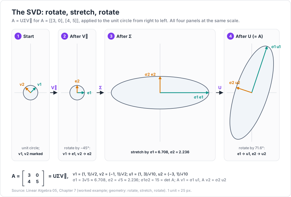
A=(3405),ATA=(25202025).
ATA has trace 50 and determinant 625−400=225, so eigenvalues 45 and 5, with unit eigenvectors v1=21(1,1) and v2=21(−1,1). The singular values are σ1=45=35≈6.708 and σ2=5≈2.236. Then
Checks: σ1σ2=15=detA (here detU=detV=1), and σ12+σ22=50=9+0+16+25, the sum of the squared entries.
Watch out: The singular values of A are not its eigenvalues. This A is triangular with eigenvalues 3 and 5, but singular values 6.708 and 2.236. For a symmetric matrix the singular values are the absolute values of the eigenvalues (more generally this holds for normal matrices, those with ATA=AAT), and for a positive semidefinite matrix they are exactly the eigenvalues.
Geometry: rotate, stretch, rotate
Read A=UΣVT from right to left as three steps applied to the unit circle:
VT is orthogonal: it rotates (or reflects) the plane, carrying v1,v2 to e1,e2. Here VT is rotation by −45°. The circle stays a circle.
Σ stretches along the axes by σ1 and σ2. The circle becomes an axis-aligned ellipse with semi-axes 6.708 and 2.236.
U rotates again, carrying e1,e2 to u1,u2. Here U is rotation by about 71.6° (the angle of (1,3)).
So every linear map of Rn sends the unit sphere to an ellipsoid (flattened when A is singular); the singular values are its semi-axes, the ui their directions, and the vi the unit vectors that land on them. In general U and V may include a reflection; both can be chosen as rotations exactly when detA≥0 (for square A).
Norms and conditioning
Spectral norm:∥A∥2=max∥x∥=1∥Ax∥=σ1 — the longest semi-axis.
Frobenius norm:∥A∥F=∑aij2=σ12+⋯+σr2 (orthogonal matrices do not change it).
Condition number of an invertible A: κ(A)=σ1/σn, the ratio of the longest to the shortest semi-axis. For the example κ=35/5=3. Solving Ax=b can amplify relative errors in b by up to κ; since σi(ATA)=σi2, forming the normal equations squares it. This, and not the size of detA, measures closeness to singularity (Linear Algebra 03, Chapter 7).
Chapter 8 — Using the SVD
Low-rank approximation
Theorem 8 (Eckart–Young, statement). Let A=∑i=1rσiuiviT and, for k<r, Ak=∑i=1kσiuiviT. Among all matrices B of rank at most k,
and ∥A−A1∥F2=2.25+2.25+0.25+0.25=5=σ22, as the theorem says.
Storage: a rank-k approximation of an m×n matrix needs k(m+n+1) numbers instead of mn. For a 1000×1000 greyscale image and k=50, that is 100050 numbers instead of 1000000, about 10%. Whether the result looks acceptable depends on how fast the singular values decay.
The pseudoinverse
The Moore–Penrose pseudoinverse of A=UΣVT is
A+=VΣ+UT,
where Σ+ is n×m with 1/σi in place of each nonzero σi. It inverts A on the row space and sends the left null space to 0. x+=A+b is the least-squares solution of Ax=b with the smallest norm — well defined even when A is rank-deficient and the normal equations have infinitely many solutions. If A has independent columns, A+=(ATA)−1AT and A+b is the x^ of Chapter 4; for the line fit, A+b=(−0.5,1.2). If A is invertible, A+=A−1.
Example.A=(1111)=2uuT with u=21(1,1), so A+=21uuT=41(1111). For b=(1,3) (not in the column space), x+=A+b=(1,1). Every x with x1+x2=2 gives the same smallest residual (because Ax=(2,2), the projection of b), and (1,1) is the shortest of them.
Principal component analysis
Put N data points in Rp as the rows of a matrix and subtract the mean of each column, giving a centred N×p matrix X. The sample covariance matrix is C=N−11XTX. If X=UΣVT then C=VN−1ΣTΣVT, so:
the principal directions are the right singular vectors vi (eigenvectors of C);
the variance along vi is σi2/(N−1);
projecting the data onto v1,…,vk is the best k-dimensional summary in the least-squares sense (Eckart–Young applied to X).
Worked example. The four points (3,3),(−3,−3),(1,−1),(−1,1) already have mean zero. XTX=(20161620) has eigenvalues 36 and 4 with eigenvectors (1,1) and (1,−1), so the singular values of X are 6 and 2. The first principal direction is 21(1,1) with variance 36/3=12; the second has variance 4/3. The first component explains 36/(36+4)=90% of the total variance.
Common pitfall: Forgetting to centre the data. Without subtracting the mean, the first "principal component" mostly points at the mean itself. Also scale the columns first when they are in different units, or the largest-unit variable dominates.
Practice Exercises
1. Show that ⟨f,g⟩=∫01f(t)g(t)dt satisfies the positive-definiteness axiom on C[0,1]. Then find the projection of f(t)=t onto the constants.
Solution
⟨f,f⟩=∫01f2≥0. If f is continuous and f(t0)=0, then f2>21f(t0)2 on some interval around t0, so the integral is positive; hence ⟨f,f⟩=0 forces f=0. (Continuity matters here.) Projection onto span(1): ⟨1,1⟩⟨t,1⟩⋅1=11/2=21. The residual t−21 is orthogonal to 1, as computed in Chapter 1.
2. Apply Gram–Schmidt to a1=(1,1,1,1), a2=(0,1,2,3).
Solution
q1=21(1,1,1,1). ⟨a2,a1⟩/⟨a1,a1⟩=6/4=23, so w2=(0,1,2,3)−23(1,1,1,1)=(−23,−21,21,23) with ∥w2∥=49+41+41+49=5. So q2=251(−3,−1,1,3). (This is the "centred x" that makes line fitting at x=0,1,2,3 decouple.)
3. For the line fit in Chapter 4, compute the projection matrix P=A(ATA)−1AT and check Pb.
Solution
(ATA)−1=201(30−10−104), and
P=101741−243211234−2147.
Pb=101(7+8+2−10,4+6+4+5,1+4+6+20,−2+2+8+35)=(0.7,1.9,3.1,4.3), the fitted values. Also P2=P and PT=P.
4. Is (4223) positive definite? Use two different tests.
Solution
Leading minors: 4>0 and 12−4=8>0: yes. Eigenvalues: trace 7, determinant 8, so λ=27±49−32=27±17, both positive because 17<7. Or complete the square: 4x2+4xy+3y2=(2x+y)2+2y2.
5. Find the singular values of E=(212−1) and its condition number.
Solution
ETE=(5335) has eigenvalues 8 and 2, so σ1=22, σ2=2, and κ=2. Check: σ1σ2=4=∣detE∣=∣−2−2∣.
6. Prove that if Q is orthogonal then every real eigenvalue of Q is ±1, and every singular value of Q is 1.
Solution
If Qv=λv with v=0, then ∥v∥=∥Qv∥=∣λ∣∥v∥, so ∣λ∣=1. Singular values are square roots of the eigenvalues of QTQ=I, all equal to 1: an orthogonal map sends the unit sphere to itself.
7. Show that for a symmetric positive semidefinite matrix the SVD and the spectral decomposition coincide, and give a 2×2 symmetric matrix where they differ.
Solution
If A=QΛQT with all λi≥0 (sorted in decreasing order), then U=V=Q and Σ=Λ is a valid SVD. For a symmetric matrix with a negative eigenvalue, such as (1221) (eigenvalues 3,−1), the singular values are 3 and 1: the sign moves into U (take u2=−v2).
Cheat-sheet
Idea
Formula or fact
Inner product
symmetric, linear, ⟨v,v⟩>0 for v=0
Cauchy–Schwarz
∣⟨u,v⟩∣≤∥u∥∥v∥
Orthonormal coordinates
v=∑⟨v,qi⟩qi
Projection
P=QQT or A(ATA)−1AT; P2=P=PT
Best approximation
PWv is the closest point of W
Gram–Schmidt
wj=vj−∑i<j⟨vj,qi⟩qi
QR
A=QR, R upper triangular
Least squares
ATAx^=ATb, or Rx^=QTb
Orthogonal matrix
QTQ=I, detQ=±1, keeps lengths
Spectral theorem
A=AT⟺A=QΛQT, real Λ
Positive definite
eigenvalues, leading minors, pivots all >0; A=RTR
Quadratic form
principal axes = eigenvectors of A
SVD
A=UΣVT, Avi=σiui, σi=λi(ATA)
Norms
∥A∥2=σ1, ∥A∥F2=∑σi2, κ=σ1/σn
Eckart–Young
best rank k: keep the top k terms; error σk+1
Pseudoinverse
A+=VΣ+UT, minimum-norm least squares
PCA
centre, SVD; variance along vi is σi2/(N−1)
What's next
This completes the base series: from solving Ax=b by elimination (post 00) to the SVD, which describes any matrix completely by two orthonormal bases and a list of stretch factors. The table below lists the posts planned to extend the series. The most natural next step is canonical forms — the full proof of the Jordan form stated in Linear Algebra 04 — followed by the numerical side, where the algorithms behind numpy.linalg (LU with pivoting, Householder QR, the QR eigenvalue algorithm, Golub–Kahan SVD) are studied for speed and accuracy.
Planned future extensions
Post
Topic
What it covers
06
Jordan form and canonical forms
generalised eigenvectors, the Jordan form proof, minimal polynomial, rational canonical form, eAt for defective matrices
07
Numerical linear algebra
floating point and conditioning, LU with pivoting, Householder QR, QR eigenvalue algorithm, computing the SVD, iterative solvers (conjugate gradient, GMRES)
08
Linear algebra for machine learning
linear regression and ridge regression, PCA in practice, matrix calculus and gradients, low-rank methods, embeddings
09
Tensors and multilinear algebra
dual spaces, bilinear forms, tensor products, exterior algebra and the determinant revisited, tensor decompositions
10
Functional analysis preview
normed and Hilbert spaces, infinite orthonormal bases and Fourier series, bounded operators, the spectral theorem for compact self-adjoint operators
References
Sheldon Axler, Linear Algebra Done Right, 4th ed., Springer (2024) — Chapter 6 (inner product spaces, Gram–Schmidt, orthogonal projection, least squares) and Chapter 7 (self-adjoint operators, the spectral theorem, positive operators, SVD). Open access at linear.axler.net.
Gilbert Strang, Introduction to Linear Algebra, 6th ed., Wellesley-Cambridge Press (2023) — orthogonality, projections, least squares, Gram–Schmidt; symmetric and positive definite matrices; the SVD and PCA.
Gilbert Strang, Linear Algebra and Learning from Data, Wellesley-Cambridge Press (2019) — the SVD, Eckart–Young, PCA and low-rank approximation from the data-science side.
Lloyd N. Trefethen, David Bau III, Numerical Linear Algebra, SIAM (1997) — Lectures 4–5 (SVD), 6–11 (projectors, QR, Gram–Schmidt, Householder, least squares), 12–15 (conditioning and stability).
Gene H. Golub, Charles F. Van Loan, Matrix Computations, 4th ed., Johns Hopkins University Press (2013) — the reference for QR, SVD and least-squares algorithms.
Roger A. Horn, Charles R. Johnson, Matrix Analysis, 2nd ed., Cambridge University Press (2012) — positive definite matrices, the spectral theorem and the SVD with complete proofs.
Carl Eckart, Gale Young, "The approximation of one matrix by another of lower rank", Psychometrika 1 (1936), 211–218 — the original low-rank approximation theorem.
Note: this post is in progress. Planned additions: complex inner product spaces and unitary matrices, the spectral theorem for normal matrices, a proof of Eckart–Young, a larger PCA example on real data with a scree plot, and a total-least-squares section.