Linear algebra is the study of vectors, of the linear equations that tie them together, and of the maps that preserve their structure. It is the working language of numerical computing, statistics, machine learning, graphics, quantum mechanics and control, and it is the first course where most students meet mathematics built from definitions and proofs rather than from formulas. This six-post series is written for a reader who knows high-school algebra and wants the full senior-undergraduate picture: computation first, then the abstract theory, with proofs of the key theorems. Post 00 starts at the very beginning — vectors in $\mathbb{R}^n$ , linear combinations, span, the dot product, systems of linear equations and Gaussian elimination — and ends with the structure of a solution set and a first look at linear independence. Posts 01–05 cover matrix algebra and LU, vector spaces and dimension, linear maps and determinants, eigenvalues, and inner products through the spectral theorem and the SVD. The standard textbooks behind the series are Strang (computation and the four subspaces), Lay (clear worked examples), Axler (the abstract, determinant-free view) and Hoffman–Kunze (the classical rigorous treatment).

Series map: 00 Vectors & Linear Systems (this post) → 01 Matrix Algebra, Inverses & LU → 02 Vector Spaces, Basis & Dimension → 03 Linear Maps, Change of Basis & Determinants → 04 Eigenvalues & Diagonalization → 05 Inner Products, Spectral Theorem & SVD.

Learning Outcome

Add and scale vectors in $\mathbb{R}^n$ , and describe a linear combination both algebraically and geometrically.
Describe the span of one, two or three vectors in $\mathbb{R}^3$ as a point, a line, a plane or all of space.
Compute dot products, lengths and angles, and recognise orthogonal vectors.
Read a system $A\mathbf{x} = \mathbf{b}$ in two ways: the row picture (intersecting lines or planes) and the column picture (a combination of columns).
Apply the three elementary row operations and explain why they never change the solution set.
Run Gaussian elimination and Gauss–Jordan elimination by hand, and bring a matrix to row echelon form and to reduced row echelon form.
Identify pivots and free variables, decide consistency, and write every solution in parametric vector form.
Prove that a solution set is "one particular solution plus all homogeneous solutions".
Test a small set of vectors for linear independence.

Notation used in the whole series

Symbol	Meaning
$\mathbb{R}$ , $\mathbb{R}^n$	real numbers; column vectors with $n$ real entries
$\mathbf{x}, \mathbf{v}, \mathbf{b}$	vectors (bold lower case), always columns unless stated
$x_i$	the $i$ -th entry of $\mathbf{x}$
$A, B, U$	matrices (capital letters); $a_{ij}$ is the entry in row $i$ , column $j$
$m \times n$	$m$ rows, $n$ columns
$\mathbf{a}_j$	column $j$ of $A$
$A^T$	transpose (rows become columns)
$\mathbf{0}$	the zero vector
$\mathbf{e}_i$	standard basis vector: 1 in position $i$ , 0 elsewhere

Chapter 1 — Vectors in n-space

Terminology

Scalar — a single real number. Later in the series scalars may come from any field (see Linear Algebra 02), but for now they are real.
Vector in $\mathbb{R}^n$ — an ordered list of $n$ real numbers, written as a column. The numbers are its entries or components.
Zero vector $\mathbf{0}$ — the vector whose entries are all 0.
Vector addition — add entry by entry. Only defined for two vectors of the same length.
Scalar multiplication — multiply every entry by the same scalar.

$\mathbf{v} = \begin{pmatrix} v_1 \\ v_2 \\ \vdots \\ v_n \end{pmatrix}, \qquad \mathbf{v} + \mathbf{w} = \begin{pmatrix} v_1 + w_1 \\ \vdots \\ v_n + w_n \end{pmatrix}, \qquad c\,\mathbf{v} = \begin{pmatrix} c v_1 \\ \vdots \\ c v_n \end{pmatrix}.$

Algebraic rules

For all $\mathbf{u}, \mathbf{v}, \mathbf{w} \in \mathbb{R}^n$ and all scalars $c, d$ :

$\mathbf{u} + \mathbf{v} = \mathbf{v} + \mathbf{u}$ and $(\mathbf{u} + \mathbf{v}) + \mathbf{w} = \mathbf{u} + (\mathbf{v} + \mathbf{w})$ .
$\mathbf{v} + \mathbf{0} = \mathbf{v}$ and $\mathbf{v} + (-\mathbf{v}) = \mathbf{0}$ .
$c(\mathbf{u} + \mathbf{v}) = c\mathbf{u} + c\mathbf{v}$ and $(c + d)\mathbf{v} = c\mathbf{v} + d\mathbf{v}$ .
$c(d\mathbf{v}) = (cd)\mathbf{v}$ and $1\mathbf{v} = \mathbf{v}$ .

Each rule follows from the matching rule for real numbers, applied one entry at a time. These eight rules are exactly the axioms of a vector space; Linear Algebra 02 turns them into a definition, and then polynomials, functions and matrices become "vectors" too.

The geometric picture

In $\mathbb{R}^2$ and $\mathbb{R}^3$ a vector is an arrow from the origin to the point with those coordinates.

Addition is the parallelogram rule: place the tail of $\mathbf{w}$ at the head of $\mathbf{v}$ ; the sum ends where $\mathbf{w}$ ends.
Scaling stretches the arrow by $\lvert c\rvert$ and reverses it when $c < 0$ .
$\mathbf{v} - \mathbf{w}$ is the arrow from the head of $\mathbf{w}$ to the head of $\mathbf{v}$ .

For $n > 3$ there is no picture, but every algebraic fact still holds. The habit to build is: reason with the algebra, check the intuition in $\mathbb{R}^2$ or $\mathbb{R}^3$ .

Watch out: a point and a vector are written the same way in $\mathbb{R}^n$ , but they play different roles. A point is a location; a vector is a displacement. The distinction matters in Chapter 7, where a solution set can be a plane that does not pass through the origin.

Chapter 2 — Linear combinations and span

Terminology

Linear combination of $\mathbf{v}_1, \dots, \mathbf{v}_k$ — any vector $c_1\mathbf{v}_1 + c_2\mathbf{v}_2 + \dots + c_k\mathbf{v}_k$ with scalars $c_1, \dots, c_k$ (the weights or coefficients).
Span — the set of all linear combinations:

$\operatorname{span}\{\mathbf{v}_1, \dots, \mathbf{v}_k\} = \{\, c_1\mathbf{v}_1 + \dots + c_k\mathbf{v}_k : c_1, \dots, c_k \in \mathbb{R} \,\}.$

The span always contains $\mathbf{0}$ (take every weight 0) and each $\mathbf{v}_i$ itself (weight 1 on it, 0 elsewhere).

Geometric picture of a span in R³

Vectors	Span
only $\mathbf{0}$	the single point $\{\mathbf{0}\}$
one nonzero $\mathbf{v}$	the line through the origin in direction $\mathbf{v}$
two vectors, neither a multiple of the other	the plane through the origin containing both
two vectors, one a multiple of the other	still only a line
three vectors not in one plane	all of $\mathbb{R}^3$
three vectors in one plane	only that plane (or a line)

The pattern "adding a vector enlarges the span only if the new vector is not already inside it" is the seed of linear independence (Chapter 8) and of dimension (Linear Algebra 02).

Worked example — is b in the span?

Is $\mathbf{b} = (1, 5)$ a combination of $\mathbf{a}_1 = (2, 1)$ and $\mathbf{a}_2 = (-1, 1)$ ? We need $x, y$ with

$x \begin{pmatrix} 2 \\ 1 \end{pmatrix} + y \begin{pmatrix} -1 \\ 1 \end{pmatrix} = \begin{pmatrix} 1 \\ 5 \end{pmatrix} \quad\Longleftrightarrow\quad \begin{aligned} 2x - y &= 1 \\ x + y &= 5. \end{aligned}$

Adding the two equations gives $3x = 6$ , so $x = 2$ and $y = 3$ . Check: $2(2,1) + 3(-1,1) = (4-3,\ 2+3) = (1, 5)$ . So $\mathbf{b}$ is in the span. In fact, since $\mathbf{a}_1$ and $\mathbf{a}_2$ are not parallel, their span is the whole plane $\mathbb{R}^2$ .

The key lesson: "is $\mathbf{b}$ in the span of these vectors?" is the same question as "does this linear system have a solution?" Everything in this post comes back to that sentence.

Chapter 3 — Dot product and length

This chapter is brief; inner products get their full treatment in Linear Algebra 05.

Definitions

Dot product: $\mathbf{u} \cdot \mathbf{v} = u_1 v_1 + u_2 v_2 + \dots + u_n v_n$ . It takes two vectors and returns a scalar.
Length (norm): $\lVert \mathbf{v} \rVert = \sqrt{\mathbf{v} \cdot \mathbf{v}} = \sqrt{v_1^2 + \dots + v_n^2}$ .
Unit vector: a vector of length 1. For $\mathbf{v} \neq \mathbf{0}$ , the vector $\mathbf{v} / \lVert \mathbf{v} \rVert$ is the unit vector in the same direction.
Orthogonal: $\mathbf{u}$ and $\mathbf{v}$ are orthogonal (perpendicular) when $\mathbf{u} \cdot \mathbf{v} = 0$ .

Properties

The dot product is symmetric ( $\mathbf{u}\cdot\mathbf{v} = \mathbf{v}\cdot\mathbf{u}$ ), linear in each argument, and positive definite: $\mathbf{v}\cdot\mathbf{v} \ge 0$ , with equality only for $\mathbf{v} = \mathbf{0}$ . Two inequalities hold for all $\mathbf{u}, \mathbf{v} \in \mathbb{R}^n$ (proofs in Linear Algebra 05):

$\lvert \mathbf{u} \cdot \mathbf{v} \rvert \le \lVert \mathbf{u} \rVert \, \lVert \mathbf{v} \rVert \quad \text{(Cauchy–Schwarz)}, \qquad \lVert \mathbf{u} + \mathbf{v} \rVert \le \lVert \mathbf{u} \rVert + \lVert \mathbf{v} \rVert \quad \text{(triangle inequality)}.$

Cauchy–Schwarz is what makes the angle formula legitimate: for nonzero vectors the ratio below lies in $[-1, 1]$ , so it is the cosine of exactly one angle $\theta \in [0, \pi]$ .

$\cos\theta = \frac{\mathbf{u}\cdot\mathbf{v}}{\lVert \mathbf{u}\rVert\,\lVert \mathbf{v}\rVert}.$

Worked example

Let $\mathbf{u} = (1, 2, 2)$ and $\mathbf{v} = (2, -2, 1)$ . Then $\lVert \mathbf{u} \rVert = \sqrt{1 + 4 + 4} = 3$ , so $\mathbf{u}/3 = (1/3, 2/3, 2/3)$ is a unit vector. And $\mathbf{u}\cdot\mathbf{v} = 2 - 4 + 2 = 0$ , so $\mathbf{u}$ and $\mathbf{v}$ are orthogonal.

Trick: the dot product gives a second reading of one equation. The equation $a_1x_1 + \dots + a_nx_n = b$ says $\mathbf{a}\cdot\mathbf{x} = b$ . When $b = 0$ , the solutions are exactly the vectors orthogonal to $\mathbf{a}$ — a line in $\mathbb{R}^2$ , a plane in $\mathbb{R}^3$ , a "hyperplane" in general.

Chapter 4 — Systems of linear equations

Terminology

Linear equation in $x_1, \dots, x_n$ — an equation $a_1x_1 + \dots + a_nx_n = b$ with constant coefficients $a_i$ and constant $b$ . No products $x_ix_j$ , no powers, no $\sin x$ .
System of linear equations — a finite list of linear equations in the same unknowns.
Solution — a vector $\mathbf{x}$ that satisfies every equation at once. The solution set is the set of all solutions.
Consistent — has at least one solution. Inconsistent — has none.
Equivalent systems — systems with the same solution set.
Coefficient matrix $A$ — the $m \times n$ array of the $a_{ij}$ . Augmented matrix $[\,A \mid \mathbf{b}\,]$ — $A$ with $\mathbf{b}$ attached as an extra column.

Matrix times vector

Write the columns of $A$ as $\mathbf{a}_1, \dots, \mathbf{a}_n$ . The product $A\mathbf{x}$ is defined as a combination of the columns, with the entries of $\mathbf{x}$ as weights:

$A\mathbf{x} = \begin{pmatrix} \mathbf{a}_1 & \mathbf{a}_2 & \cdots & \mathbf{a}_n \end{pmatrix} \begin{pmatrix} x_1 \\ \vdots \\ x_n \end{pmatrix} = x_1\mathbf{a}_1 + x_2\mathbf{a}_2 + \dots + x_n\mathbf{a}_n.$

Entry $i$ of that combination is $a_{i1}x_1 + \dots + a_{in}x_n$ , which is the dot product of row $i$ of $A$ with $\mathbf{x}$ . So there are two ways to compute $A\mathbf{x}$ — by columns and by rows — and they always agree. A system of $m$ equations in $n$ unknowns is therefore one vector equation $A\mathbf{x} = \mathbf{b}$ , with $A$ of size $m \times n$ , $\mathbf{x} \in \mathbb{R}^n$ and $\mathbf{b} \in \mathbb{R}^m$ .

Two rules follow straight from the definition and are used constantly: $A(\mathbf{u} + \mathbf{v}) = A\mathbf{u} + A\mathbf{v}$ and $A(c\mathbf{u}) = c\,A\mathbf{u}$ .

Row picture and column picture

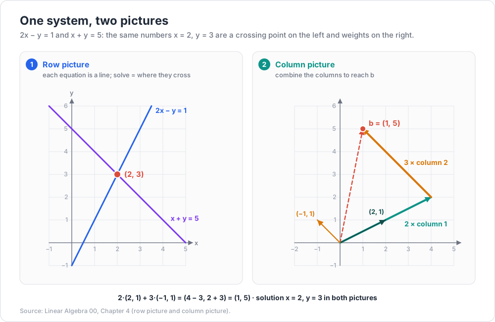
Take the system from Chapter 2:

$\begin{aligned} 2x - y &= 1 \\ x + y &= 5 \end{aligned} \qquad\Longleftrightarrow\qquad \begin{pmatrix} 2 & -1 \\ 1 & 1 \end{pmatrix} \begin{pmatrix} x \\ y \end{pmatrix} = \begin{pmatrix} 1 \\ 5 \end{pmatrix}.$

Row picture. Each equation is a line in the $xy$ -plane: $y = 2x - 1$ and $y = 5 - x$ . A solution is a point on both lines. They cross at $(2, 3)$ .
Column picture. The same system asks for weights on the columns $(2, 1)$ and $(-1, 1)$ that produce $(1, 5)$ . The answer is $2$ of the first column plus $3$ of the second.

The same numbers $x = 2$ , $y = 3$ appear in both pictures, but they mean different things: a point where lines cross, or weights in a combination.

Row picture and column picture of the system 2x − y = 1, x + y = 5: on the left the two lines cross at the point (2, 3); on the right 2 times column (2, 1) plus 3 times column (−1, 1) reaches b = (1, 5)

In $\mathbb{R}^3$ the row picture has three planes, and a solution is a point common to all three. The column picture has three column vectors in $\mathbb{R}^3$ , and the question is whether $\mathbf{b}$ is a combination of them. The column picture scales to any size and becomes the main point of view from Linear Algebra 02 onwards (column space).

How many solutions can there be?

Theorem (zero, one or infinitely many). A linear system has either no solution, exactly one solution, or infinitely many solutions.

Proof. Suppose $\mathbf{x}$ and $\mathbf{y}$ are two different solutions, so $A\mathbf{x} = A\mathbf{y} = \mathbf{b}$ . For every real $t$ , put $\mathbf{z}_t = \mathbf{x} + t(\mathbf{y} - \mathbf{x})$ . Then

$A\mathbf{z}_t = A\mathbf{x} + t(A\mathbf{y} - A\mathbf{x}) = \mathbf{b} + t(\mathbf{b} - \mathbf{b}) = \mathbf{b}.$

Since $\mathbf{y} - \mathbf{x} \neq \mathbf{0}$ , different values of $t$ give different vectors $\mathbf{z}_t$ , so there are infinitely many solutions. $\blacksquare$

Geometrically: the whole line through two solutions consists of solutions. Two lines in the plane cannot meet in exactly two points.

Chapter 5 — Elimination

Elementary row operations

Three operations on the rows of an augmented matrix:

Replacement — add a multiple of one row to another row: $R_i \leftarrow R_i + cR_j$ (with $i \neq j$ ).
Interchange — swap two rows: $R_i \leftrightarrow R_j$ .
Scaling — multiply a row by a nonzero constant: $R_i \leftarrow cR_i$ , $c \neq 0$ .

Two matrices are row equivalent if one can be turned into the other by a finite sequence of these operations.

Theorem. If two augmented matrices are row equivalent, the corresponding systems have the same solution set.

Proof. It is enough to check one operation at a time. Any $\mathbf{x}$ that satisfies the old equations also satisfies the new ones: a swap or a scaling changes nothing essential, and if $\mathbf{x}$ satisfies equations $i$ and $j$ it satisfies their sum " $i + c\cdot j$ ". Conversely, each operation can be undone by an operation of the same type — replacement by $R_i \leftarrow R_i - cR_j$ , interchange by the same swap, scaling by $1/c$ (this is why $c \neq 0$ is required). So any solution of the new system also solves the old one. $\blacksquare$

Common pitfall: multiplying a row by $0$ is not allowed. It destroys an equation and can create new "solutions". Scaling needs $c \neq 0$ precisely so the step is reversible.

Gaussian elimination on a 3 × 3 system

Solve

$\begin{aligned} x + 2y + z &= 2 \\ 3x + 8y + z &= 12 \\ 4y + z &= 2 \end{aligned} \qquad [\,A \mid \mathbf{b}\,] = \left(\begin{array}{ccc|c} 1 & 2 & 1 & 2 \\ 3 & 8 & 1 & 12 \\ 0 & 4 & 1 & 2 \end{array}\right).$

Step 1 — clear column 1 below the first pivot. The first pivot is the 1 in position (1,1). Row 2 needs multiplier $\ell_{21} = 3/1 = 3$ ; row 3 already has a 0, so $\ell_{31} = 0$ .

$R_2 \leftarrow R_2 - 3R_1: \qquad \left(\begin{array}{ccc|c} 1 & 2 & 1 & 2 \\ 0 & 2 & -2 & 6 \\ 0 & 4 & 1 & 2 \end{array}\right).$

Step 2 — clear column 2 below the second pivot. The second pivot is 2 in position (2,2). Multiplier $\ell_{32} = 4/2 = 2$ .

$R_3 \leftarrow R_3 - 2R_2: \qquad \left(\begin{array}{ccc|c} 1 & 2 & 1 & 2 \\ 0 & 2 & -2 & 6 \\ 0 & 0 & 5 & -10 \end{array}\right).$

The coefficient part is now upper triangular, with pivots $1, 2, 5$ .

Step 3 — back substitution. From the bottom up: $5z = -10$ gives $z = -2$ . Then $2y - 2z = 6$ gives $2y = 2$ , so $y = 1$ . Then $x + 2y + z = 2$ gives $x = 2 - 2 + 2 = 2$ .

Check in the original equations: $2 + 2 - 2 = 2$ , $6 + 8 - 2 = 12$ , $4 - 2 = 2$ . The unique solution is $(x, y, z) = (2, 1, -2)$ .

The multipliers $3, 0, 2$ are not thrown away in practice — Linear Algebra 01 stores them in a lower triangular matrix $L$ and gets the factorization $A = LU$ .

When elimination breaks down

Zero in a pivot position, nonzero below it — swap rows and continue. This is a temporary breakdown.
Zero in a pivot position and zeros all the way down — there is no pivot in that column. The matrix is singular (Linear Algebra 01) and the system has either no solution or infinitely many. Chapter 6 handles this case completely.

Watch out: on a computer, a pivot that is merely small is as dangerous as a zero one, because dividing by it magnifies rounding error. Software therefore swaps in the largest available entry of the column (partial pivoting). By hand, with exact numbers, any nonzero pivot is fine.

Chapter 6 — Echelon forms, pivots and free variables

Terminology

Leading entry of a row — its leftmost nonzero entry.
Row echelon form (REF) — (i) all zero rows are at the bottom; (ii) each leading entry is in a column to the right of the leading entry of the row above; (iii) all entries below a leading entry are zero.
Reduced row echelon form (RREF) — REF, plus (iv) every leading entry is 1, and (v) each leading 1 is the only nonzero entry in its column.
Pivot position — a position that holds a leading entry in an echelon form of the matrix. Pivot column — a column containing a pivot position.
Basic variable — a variable whose column is a pivot column. Free variable — any other variable.

Gauss–Jordan elimination continues past REF: scale each pivot to 1, then clear the entries above each pivot, working from the bottom pivot up.

Uniqueness of the RREF

Theorem. Each matrix is row equivalent to one and only one matrix in reduced row echelon form.

Existence is the Gauss–Jordan algorithm. Uniqueness takes a careful induction on the number of columns; see Lay, Appendix A, or Hoffman–Kunze, Chapter 1. It has an important consequence: the pivot positions — and so the pivot columns, the number of pivots and the split into basic and free variables — do not depend on which row operations you chose. An REF is not unique (you can always scale a row by 2), but its pivot positions are.

A worked 3 × 4 example

Solve $A\mathbf{x} = \mathbf{b}$ with

$A = \begin{pmatrix} 1 & 2 & 2 & 2 \\ 2 & 4 & 6 & 8 \\ 3 & 6 & 8 & 10 \end{pmatrix}, \qquad \mathbf{b} = \begin{pmatrix} 1 \\ 6 \\ 7 \end{pmatrix}.$

Forward elimination, $R_2 \leftarrow R_2 - 2R_1$ and $R_3 \leftarrow R_3 - 3R_1$ :

$\left(\begin{array}{cccc|c} 1 & 2 & 2 & 2 & 1 \\ 0 & 0 & 2 & 4 & 4 \\ 0 & 0 & 2 & 4 & 4 \end{array}\right).$

Column 2 has no pivot (zeros from row 2 down), so move to column 3; its pivot is the 2 in row 2. Then $R_3 \leftarrow R_3 - R_2$ :

$\left(\begin{array}{cccc|c} 1 & 2 & 2 & 2 & 1 \\ 0 & 0 & 2 & 4 & 4 \\ 0 & 0 & 0 & 0 & 0 \end{array}\right) \quad \text{(REF)}.$

Gauss–Jordan: $R_2 \leftarrow \tfrac12 R_2$ , then $R_1 \leftarrow R_1 - 2R_2$ :

$\left(\begin{array}{cccc|c} 1 & 2 & 0 & -2 & -3 \\ 0 & 0 & 1 & 2 & 2 \\ 0 & 0 & 0 & 0 & 0 \end{array}\right) \quad \text{(RREF)}.$

Pivot columns are 1 and 3, so $x_1, x_3$ are basic and $x_2, x_4$ are free. The RREF reads

$x_1 = -3 - 2x_2 + 2x_4, \qquad x_3 = 2 - 2x_4, \qquad x_2, x_4 \text{ free}.$

Parametric vector form

Write the free variables as parameters $x_2 = s$ , $x_4 = t$ and collect terms:

$\mathbf{x} = \begin{pmatrix} x_1 \\ x_2 \\ x_3 \\ x_4 \end{pmatrix} = \begin{pmatrix} -3 \\ 0 \\ 2 \\ 0 \end{pmatrix} + s \begin{pmatrix} -2 \\ 1 \\ 0 \\ 0 \end{pmatrix} + t \begin{pmatrix} 2 \\ 0 \\ -2 \\ 1 \end{pmatrix}, \qquad s, t \in \mathbb{R}.$

The solution set is a 2-dimensional plane inside $\mathbb{R}^4$ , one parameter per free variable. Check the first vector: $A(-3, 0, 2, 0) = (-3 + 4,\ -6 + 12,\ -9 + 16) = (1, 6, 7) = \mathbf{b}$ .

Consistency

The zero row of the augmented RREF above ended in 0, so it said $0 = 0$ — harmless. Change $\mathbf{b}$ to $(1, 6, 8)$ and the same steps end with the row $(0\ 0\ 0\ 0 \mid 1)$ , which says $0 = 1$ . That system is inconsistent. In general:

Theorem (existence and uniqueness). A linear system is consistent if and only if the last column of its augmented matrix is not a pivot column — that is, no echelon form has a row $(0\ \cdots\ 0 \mid c)$ with $c \neq 0$ . If it is consistent, then it has exactly one solution when there are no free variables, and infinitely many when there is at least one free variable.

Proof. Row operations do not change the solution set, so study the RREF. A row $(0 \cdots 0 \mid c)$ with $c \neq 0$ is the equation $0 = c$ , which nothing satisfies. If there is no such row, every nonzero row of the RREF has a leading 1 in a coefficient column and expresses one basic variable in terms of the free ones; choosing any values for the free variables produces a solution. With no free variables that solution is forced and unique; with at least one free variable each choice of its value gives a different solution. $\blacksquare$

For $\mathbf{b} = (b_1, b_2, b_3)$ and our $A$ , the condition works out to $b_3 = b_1 + b_2$ : row 3 of $A$ is row 1 plus row 2, so the right-hand sides must obey the same relation.

Trick: count before you compute. If $A$ is $m \times n$ and has $r$ pivots, then $r \le m$ and $r \le n$ , and there are $n - r$ free variables. Here $m = 3$ , $n = 4$ , $r = 2$ : two free variables, and a solution for $\mathbf{b}$ only when $\mathbf{b}$ passes one test (one zero row).

Chapter 7 — Homogeneous systems and the shape of the solution set

Terminology

Homogeneous system — $A\mathbf{x} = \mathbf{0}$ . It always has the trivial solution $\mathbf{x} = \mathbf{0}$ .
Nontrivial solution — a solution $\mathbf{x} \neq \mathbf{0}$ .

Theorem. A homogeneous system with more unknowns than equations ( $n > m$ ) has a nontrivial solution.

Proof. There are at most $m$ pivots, one per row, so at least $n - m > 0$ variables are free. The system is consistent (it has $\mathbf{0}$ ), so by the existence-and-uniqueness theorem it has infinitely many solutions, and in particular a nonzero one. $\blacksquare$

For the $3 \times 4$ matrix above, $A\mathbf{x} = \mathbf{0}$ has the same RREF with a zero last column, and its solutions are

$\mathbf{x} = s \begin{pmatrix} -2 \\ 1 \\ 0 \\ 0 \end{pmatrix} + t \begin{pmatrix} 2 \\ 0 \\ -2 \\ 1 \end{pmatrix}.$

The two vectors are the special solutions: set one free variable to 1, the others to 0, and solve. This set is a plane through the origin — the null space of $A$ , studied in Linear Algebra 02.

Particular plus homogeneous

Theorem. Suppose $A\mathbf{x}_p = \mathbf{b}$ . Then the solution set of $A\mathbf{x} = \mathbf{b}$ is exactly

$\{\, \mathbf{x}_p + \mathbf{x}_h : A\mathbf{x}_h = \mathbf{0} \,\}.$

Proof. If $A\mathbf{x}_h = \mathbf{0}$ then $A(\mathbf{x}_p + \mathbf{x}_h) = \mathbf{b} + \mathbf{0} = \mathbf{b}$ . Conversely, if $A\mathbf{x} = \mathbf{b}$ , put $\mathbf{x}_h = \mathbf{x} - \mathbf{x}_p$ ; then $A\mathbf{x}_h = \mathbf{b} - \mathbf{b} = \mathbf{0}$ and $\mathbf{x} = \mathbf{x}_p + \mathbf{x}_h$ . $\blacksquare$

Compare with the parametric form in Chapter 6: $(-3, 0, 2, 0)$ is a particular solution, and the $s$ and $t$ terms are exactly the homogeneous solutions. Geometrically, the solution set of $A\mathbf{x} = \mathbf{b}$ is the null-space plane shifted by $\mathbf{x}_p$ — parallel to it, but not through the origin (unless $\mathbf{b} = \mathbf{0}$ ).

Common pitfall: the solution set of $A\mathbf{x} = \mathbf{b}$ with $\mathbf{b} \neq \mathbf{0}$ is not closed under addition: if $A\mathbf{x} = A\mathbf{y} = \mathbf{b}$ then $A(\mathbf{x} + \mathbf{y}) = 2\mathbf{b}$ . Only the homogeneous solution set is a "subspace". The particular solution is not unique either — any solution can play that role.

This is the same structure as linear differential equations ("general solution = particular solution + solution of the homogeneous equation"), and for the same reason: the operator is linear.

Chapter 8 — Linear independence, a first look

Terminology

Linearly independent — vectors $\mathbf{v}_1, \dots, \mathbf{v}_k$ such that the only solution of $c_1\mathbf{v}_1 + \dots + c_k\mathbf{v}_k = \mathbf{0}$ is $c_1 = \dots = c_k = 0$ .
Linearly dependent — not independent: some combination with not all weights zero gives $\mathbf{0}$ . Such an equation is a linear dependence relation.

Put the vectors as the columns of $A$ . Then $c_1\mathbf{v}_1 + \dots + c_k\mathbf{v}_k = A\mathbf{c}$ , so:

The columns of $A$ are linearly independent $\iff$ $A\mathbf{c} = \mathbf{0}$ has only the trivial solution $\iff$ every column of $A$ is a pivot column (no free variables).

Worked example

Are $\mathbf{v}_1 = (1, 2, 3)$ , $\mathbf{v}_2 = (4, 5, 6)$ , $\mathbf{v}_3 = (7, 8, 9)$ independent? Row reduce

$\begin{pmatrix} 1 & 4 & 7 \\ 2 & 5 & 8 \\ 3 & 6 & 9 \end{pmatrix} \to \begin{pmatrix} 1 & 4 & 7 \\ 0 & -3 & -6 \\ 0 & -6 & -12 \end{pmatrix} \to \begin{pmatrix} 1 & 4 & 7 \\ 0 & -3 & -6 \\ 0 & 0 & 0 \end{pmatrix}.$

Column 3 is not a pivot column, so the vectors are dependent. The free variable $c_3 = 1$ gives $-3c_2 - 6 = 0$ , so $c_2 = -2$ , and $c_1 + 4(-2) + 7 = 0$ , so $c_1 = 1$ . The dependence relation is

$\mathbf{v}_1 - 2\mathbf{v}_2 + \mathbf{v}_3 = \mathbf{0}.$

Check: $(1 - 8 + 7,\ 2 - 10 + 8,\ 3 - 12 + 9) = (0, 0, 0)$ . Geometrically, the three vectors lie in one plane through the origin, so their span is that plane, not all of $\mathbb{R}^3$ .

Quick facts

Theorem.

Any set containing $\mathbf{0}$ is dependent ( $1\cdot\mathbf{0} = \mathbf{0}$ is a nontrivial relation).
Two vectors are dependent if and only if one is a scalar multiple of the other.
A set of vectors is dependent if and only if at least one of them is a linear combination of the others.
More than $n$ vectors in $\mathbb{R}^n$ are always dependent.

Proof of 3. If $c_1\mathbf{v}_1 + \dots + c_k\mathbf{v}_k = \mathbf{0}$ with some $c_j \neq 0$ , divide by $c_j$ and solve for $\mathbf{v}_j$ in terms of the others. Conversely, if $\mathbf{v}_j = \sum_{i \neq j} d_i\mathbf{v}_i$ , then $\sum_{i \neq j} d_i\mathbf{v}_i - \mathbf{v}_j = \mathbf{0}$ is a relation with weight $-1 \neq 0$ on $\mathbf{v}_j$ . Statement 2 is the case $k = 2$ .

Proof of 4. With $k > n$ vectors as columns, $A$ is $n \times k$ with more unknowns than equations, so by the Chapter 7 theorem $A\mathbf{c} = \mathbf{0}$ has a nontrivial solution. $\blacksquare$

Watch out: statement 3 says some vector is a combination of the others, not every vector. In $\{(1,0), (2,0), (0,1)\}$ the first two are dependent, but $(0,1)$ is not a combination of them.

Linear Algebra 02 makes independence and span precise in any vector space and combines them into the idea of a basis.

Practice Exercises

Exercise 1 — Span

Is $\mathbf{b} = (3, 1, 2)$ in the span of $\mathbf{v}_1 = (1, 0, 1)$ and $\mathbf{v}_2 = (1, 1, 0)$ ? If yes, give the weights.

Solution

Solve $x(1,0,1) + y(1,1,0) = (3,1,2)$ : the equations are $x + y = 3$ , $y = 1$ , $x = 2$ . They agree: $x = 2$ , $y = 1$ . So $\mathbf{b} = 2\mathbf{v}_1 + \mathbf{v}_2$ , and $\mathbf{b}$ is in the span. (Three equations, two unknowns: consistency was not guaranteed; with $\mathbf{b} = (3, 1, 3)$ it would fail.)

Exercise 2 — Dot product

Find a unit vector in the direction of $(2, -1, 2)$ and a nonzero vector orthogonal to it.

Solution

The length is $\sqrt{4 + 1 + 4} = 3$ , so the unit vector is $(2/3, -1/3, 2/3)$ . Any $(a, b, c)$ with $2a - b + 2c = 0$ is orthogonal, for example $(1, 2, 0)$ : $2 - 2 + 0 = 0$ .

Exercise 3 — Elimination

Solve by Gaussian elimination and back substitution: $x + y + z = 6$ , $2x + 3y + z = 11$ , $x + 2y + 3z = 14$ .

Solution

$R_2 \leftarrow R_2 - 2R_1$ gives $(0, 1, -1 \mid -1)$ . $R_3 \leftarrow R_3 - R_1$ gives $(0, 1, 2 \mid 8)$ . $R_3 \leftarrow R_3 - R_2$ gives $(0, 0, 3 \mid 9)$ . Back substitution: $z = 3$ ; $y - 3 = -1$ so $y = 2$ ; $x + 2 + 3 = 6$ so $x = 1$ . Pivots $1, 1, 3$ . Check: $2 + 6 + 3 = 11$ and $1 + 4 + 9 = 14$ .

Exercise 4 — RREF and parametric form

Bring $\left(\begin{array}{ccc|c} 1 & -1 & 2 & 3 \\ 2 & -2 & 5 & 8 \end{array}\right)$ to RREF and write the solution set in parametric vector form.

Solution

$R_2 \leftarrow R_2 - 2R_1$ gives $(0, 0, 1 \mid 2)$ . Then $R_1 \leftarrow R_1 - 2R_2$ gives $(1, -1, 0 \mid -1)$ . Pivot columns 1 and 3; $x_2 = s$ is free. So $x_1 = -1 + s$ , $x_3 = 2$ :

$\mathbf{x} = \begin{pmatrix} -1 \\ 0 \\ 2 \end{pmatrix} + s \begin{pmatrix} 1 \\ 1 \\ 0 \end{pmatrix}.$

A line in $\mathbb{R}^3$ that does not pass through the origin.

Exercise 5 — Consistency condition

For which $h$ is the system $x + 2y = 4$ , $3x + 6y = h$ consistent? How many solutions does it have then?

Solution

$R_2 \leftarrow R_2 - 3R_1$ gives $(0, 0 \mid h - 12)$ . Consistent exactly when $h = 12$ . Then $y$ is free and there are infinitely many solutions, $x = 4 - 2y$ . In the row picture the two lines are parallel, and they coincide only when $h = 12$ .

Exercise 6 — Independence

Are $(1, 1, 0)$ , $(0, 1, 1)$ , $(1, 0, 1)$ linearly independent? What is their span?

Solution

Row reduce the matrix with these columns: $\begin{pmatrix} 1 & 0 & 1 \\ 1 & 1 & 0 \\ 0 & 1 & 1 \end{pmatrix} \to \begin{pmatrix} 1 & 0 & 1 \\ 0 & 1 & -1 \\ 0 & 1 & 1 \end{pmatrix} \to \begin{pmatrix} 1 & 0 & 1 \\ 0 & 1 & -1 \\ 0 & 0 & 2 \end{pmatrix}$ . Three pivots, so the columns are independent. Every row has a pivot too, so $A\mathbf{x} = \mathbf{b}$ is solvable for every $\mathbf{b}$ : the span is all of $\mathbb{R}^3$ .

Exercise 7 — Proof

Prove: if $\mathbf{u}$ and $\mathbf{v}$ both solve $A\mathbf{x} = \mathbf{0}$ , then so does every linear combination $c\mathbf{u} + d\mathbf{v}$ . Does the same hold for $A\mathbf{x} = \mathbf{b}$ with $\mathbf{b} \neq \mathbf{0}$ ?

Solution

$A(c\mathbf{u} + d\mathbf{v}) = cA\mathbf{u} + dA\mathbf{v} = c\mathbf{0} + d\mathbf{0} = \mathbf{0}$ . For $\mathbf{b} \neq \mathbf{0}$ it fails: $A(c\mathbf{u} + d\mathbf{v}) = (c + d)\mathbf{b}$ , which equals $\mathbf{b}$ only when $c + d = 1$ . (Combinations with weights summing to 1 are called affine combinations; they are exactly what the Chapter 4 proof used.)

Cheat-sheet

Idea	Key fact
Linear combination	$c_1\mathbf{v}_1 + \dots + c_k\mathbf{v}_k$
Span	all linear combinations; always contains $\mathbf{0}$
$A\mathbf{x}$	$x_1\mathbf{a}_1 + \dots + x_n\mathbf{a}_n$ (columns), or row $i$ dot $\mathbf{x}$ (rows)
$\mathbf{b}$ in span of columns	$\iff$ $A\mathbf{x} = \mathbf{b}$ is consistent
Length, angle	$\lVert\mathbf{v}\rVert = \sqrt{\mathbf{v}\cdot\mathbf{v}}$ ; $\cos\theta = \mathbf{u}\cdot\mathbf{v} / (\lVert\mathbf{u}\rVert\lVert\mathbf{v}\rVert)$
Row operations	replace, swap, scale by $c \neq 0$ — all reversible
Number of solutions	0, 1 or infinitely many
REF vs RREF	REF not unique; RREF unique; pivot positions unique
Inconsistent	a row $(0 \cdots 0 \mid c)$ with $c \neq 0$
Free variables	$n - r$ for $r$ pivots; each gives one parameter
Homogeneous, $n > m$	always a nontrivial solution
Solution set	$\mathbf{x}_p$ + (all solutions of $A\mathbf{x} = \mathbf{0}$ )
Columns independent	$\iff$ a pivot in every column
More than $n$ vectors in $\mathbb{R}^n$	always dependent

What's next

Linear Algebra 01 treats matrices as objects in their own right. It multiplies them four different ways, explains why $AB \neq BA$ , writes each row operation as an elementary matrix, defines the inverse and computes it by Gauss–Jordan, lists the first equivalent conditions for invertibility, and turns the elimination in Chapter 5 into the factorization $A = LU$ — the form in which every serious linear solver actually works.

References

Gilbert Strang, Introduction to Linear Algebra, 6th edition, Wellesley-Cambridge Press, 2023 — Chapters 1–2 (vectors, the row and column pictures, elimination). Book site: math.mit.edu/linearalgebra.
David C. Lay, Steven R. Lay and Judi J. McDonald, Linear Algebra and Its Applications, 6th edition, Pearson, 2021 — Chapter 1 (row reduction, echelon forms, solution sets, linear independence); Appendix A proves uniqueness of the RREF.
Sheldon Axler, Linear Algebra Done Right, 4th edition, Springer (Undergraduate Texts in Mathematics), 2024 — open access at linear.axler.net. Chapter 1 for $\mathbb{R}^n$ and $\mathbb{F}^n$ .
Kenneth Hoffman and Ray Kunze, Linear Algebra, 2nd edition, Prentice-Hall, 1971 — Chapter 1 (linear equations, row-reduced echelon matrices).
MIT OpenCourseWare, 18.06 Linear Algebra, Spring 2010 (Gilbert Strang) — Lectures 1–2: the geometry of linear equations, elimination with matrices.

Note: this post is in progress. Planned additions: a short section on the geometry of three planes in $\mathbb{R}^3$ (all the ways they can fail to meet), an operation count for elimination by hand, and a worked example of partial pivoting with rounding to three digits.