
MongoDB Course — 18 · Mongoose Deep Dive (Schemas, Hooks, Populate, Discriminators, Plugins, Transactions)
Mongoose has been the dominant Node.js ODM for MongoDB since 2012; in 2026 it's at v9.x. Post 17 introduced it briefly; this post is the working deep-dive — every schema feature you'll actually use, validation, hooks (pre/post middleware), virtuals, getters/setters, methods + statics, populate + strategies, discriminators (single-collection inheritance), plugins, transactions inside Mongoose, performance traps (), and when to ditch it for the official driver + Zod.
> Series map: 00 → 17 base course → 18 Mongoose Deep (this post) → 19 Beanie + FastAPI → 20 Outbox → 21 CQRS + ES → 22 RAG → 23 SQL→Mongo migration → 24 Kafka + Debezium CDC → 25 Testing → 26 OpenTelemetry → 27 Geo deep → 28 Time-series extreme → 29 K8s + mongosync + cost + compliance.
Learning Outcome
- Define Mongoose schemas with every common option (types, defaults, validators, indexes).- Use pre/post hooks idiomatically.- Add virtuals, getters/setters, methods, statics, query helpers.- Use with paths, multi-step, conditions; understand its costs.- Use discriminators for polymorphic collections.- Build + apply plugins.- Run Mongoose transactions with .- Apply and other performance escape hatches.
Chapter 1 — Connect + bootstrap
is a singleton wrapper around . Sharing connections + pool across the whole app is automatic.
Chapter 2 — Schemas
Schema type shorthand: is equivalent to .
Built-in types
, , , , , (), , , , (any), (8.x+).
Schema-level options worth knowing
| Option | Effect ||--------|--------|| | auto + || | error on unknown fields (default: silently strip) || | omit || | use for safer save() concurrency || | override default || | disable virtual getter (string of ) || | include virtuals when serialising |
Chapter 3 — Validators
Built-in: , , , , , , .
Custom synchronous:
Custom async:
Run validators on :
By default validators run only on . Always pass when using if you want validation enforced.
Chapter 4 — Hooks (pre / post middleware)
Hooks fire around , , , , , , , and more.
Document middleware (, , , ) — is the document.Query middleware (, , etc.) — is the query, not the doc:
Aggregation middleware:
Pitfalls
- hooks don't fire middleware. Use the hook explicitly.- ops skip hooks unless you opt in.- Throw inside to abort the op.- can't reject the operation — for side-effect-only work.
Chapter 5 — Virtuals, getters, setters
Virtuals aren't persisted. Include in JSON output with .
Getters / setters transform field values on read / write:
Caveat: getters don't run inside calls. Setters run on assignment + .
Chapter 6 — Methods, statics, query helpers
Keep models tidy by attaching domain logic here.
Chapter 7 — Populate (the Mongoose "join")
Multi-step:
Conditional populate:
Cost
runs additional queries — one per referenced collection, with over the gathered IDs. Not server-side — happens client-side via the driver.
When you have many populates over big lists, prefer:
1. Embedded references — denormalise the rare fields you always need (Post 07 extended-reference pattern).2. Aggregation — single round-trip server-side.
> Trick: lint for populates inside loops. Each iteration is a fresh round-trip. Always fan out the IDs first, then one , then map.
Chapter 8 — Discriminators (polymorphic collection)
Single collection holds multiple subtypes:
The discriminator key is stored on each doc ( or ). Queries on the subtype model auto-filter.
Use for the polymorphic pattern (Post 07). Cleaner than manual field handling in the app.
Embedded discriminators work too — array of mixed-type sub-documents.
Chapter 9 — Plugins
Plugins add cross-cutting schema features. Pattern:
Useful community plugins
| Plugin | Use ||--------|-----|| | cursor + offset pagination helpers || | auto on configured fields || | paginate aggregation results || | nicer error on unique violation || | field-level encryption (CSFLE alternative) || | revision log per doc || | soft-delete out-of-the-box || | preserve virtuals in output |
Apply globally: before any model registration.
Chapter 10 — Transactions in Mongoose
Pass to every Mongoose op inside. Same rules + retry semantics as the official-driver pattern (Post 09).
Note — array form is required when passing options to .
Chapter 11 — — the perf escape hatch
By default Mongoose returns Mongoose documents — heavy objects with getters, virtuals, change tracking, methods.
For read-only queries (API responses, dashboards), use :
Faster by 2-10× on big result sets. Loses: virtuals (use ), getters, checks, methods, change tracking.
Rule: default on every list endpoint. Skip it only when you're going to mutate + save.
Chapter 12 — Indexes + Mongoose
Schema-level:
On startup, Mongoose calls for each model. In production, disable auto-indexing + create indexes through migrations:
Auto-indexing blocks reads/writes on first run with a big collection. Always control index builds explicitly in production.
Chapter 13 — Subdocuments + arrays
Subdocument arrays are validated + middleware-aware. Use them for bounded 1:few children (Post 07).
Chapter 14 — Schema-less / mixed types
When a field genuinely has dynamic shape:
For SaaS multi-tenant where each tenant has custom fields, prefer the attribute pattern (Post 07) over .
Chapter 15 — Mongoose vs official driver + Zod
| Aspect | Mongoose | Official + Zod ||--------|----------|----------------|| Schema + validation | rich, in-DB-friendly | runtime validation only || Middleware (hooks) | yes | none built-in (wrap manually) || | client-side joins free | use aggregation || Type safety in TypeScript | inferred but partial | full inference via Zod || Performance | 30-50 % slower than driver | matches driver || Aggregation | thin wrapper | identical to driver || Discriminators | nice | manual field || Community | huge | thinner |
Pick Mongoose for: traditional Express/Node services, teams used to ORM-style codebases, lots of populate use.
Pick official + Zod for: TypeScript-first projects, edge runtimes, services where aggregation is hot path, microservices that want minimal dependencies.
Both run perfectly fine on the same DB. You can mix per service.
Chapter 16 — Common pitfalls
| Pitfall | Cause | Fix ||---------|-------|-----|| Validators not running on update | default: only runs them | || round-trips per loop iter | N+1 query problem | batch IDs, single query || field changes not saved | Mongoose can't detect nested change | || Heavy responses on list endpoints | not using | add || Production startup slow / blocking | rebuild on big collection | disable in prod; migrate indexes manually || Hooks fire twice on same op | both pre('save') + pre('updateOne') registered | pick one per op || returns old doc | default behaviour | || Discriminator queries on base also return subtype | by design; filter explicitly if needed | || Schema circular ref errors | two schemas reference each other before model registered | declare schemas first, register models after |
Practice Exercises
Exercise 1 — Soft-delete plugin
Build the soft-delete plugin from Chapter 9. Apply to + . Confirm queries auto-filter, works.
Exercise 2 — Populate vs $lookup benchmark
Build the post-with-author relationship. Fetch 100 posts with vs an aggregation . Measure latency.
Exercise 3 — Discriminators
Create base + + discriminators. Insert mixed events. Query both with the base model + each subtype.
Exercise 4 — Transactions
Implement the function from Chapter 10. Test the insufficient-funds rollback.
Exercise 5 — Hooks chain
Add a hook hashing passwords, a hook publishing an event, and a soft-delete filter. Verify all fire correctly.
Exercise 6 — mass conversion
Take any list endpoint in a Mongoose app. Add . Measure p95 latency before vs after.
Cheat-sheet
| What | How ||------|-----|| Connect | || Define schema | || Index | || Validator | || Pre/post hook | / || Query middleware | (this = query) || Virtual | || Method (instance) | || Static (model) | || Query helper | || Populate | or pipeline form || Discriminator | || Plugin | or global || Transaction | || Pass session | to every op || Perf escape | for read-only || Production index | ; migrate manually || Soft delete | plugin + query middleware filter || Update validation | || Get new doc post-update | || Mongoose v current | 9.x (2026) |
What's next
Post 19 covers Beanie + Pydantic v2 + FastAPI — the Python equivalent of Mongoose's ergonomics, integrated with the dominant Python web stack.
References
- Mongoose docs- Mongoose Schemas Guide- Mongoose Discriminators- Mongoose Plugins- Mongoose ODM Support (MongoDB Inc)
> Note: this post is in progress. Planned additions: Mongoose 9 changelog highlights; integration with NestJS; comparison with ; perf benchmarks.
MongoDB Course — 17 · Drivers + Modeling Case Studies (Time-Series, IoT, E-commerce, Social, Multi-Tenant)
The final base post wraps up the series with two practical halves. First — a quick tour of the major drivers (Node official + Mongoose vs Prisma, Python pymongo + Motor, Go, Rust, .NET) so you can match idioms to the language you actually ship in. Second — end-to-end modelling case studies for the five workloads that show up most often: native time-series collections, IoT telemetry, e-commerce catalogue + orders, social feed, and multi-tenant SaaS.
> Series map: 00 Foundations → … → 16 Atlas → 17 Drivers & Case Studies (this post — final base).
Learning Outcome
- Use the official Node driver + know when to layer Mongoose vs Prisma.- Switch idioms between pymongo / Motor for sync vs async Python.- Recognise driver patterns in Go, Rust, .NET.- Apply native time-series collections correctly.- Model IoT telemetry, e-commerce, social feed, multi-tenant SaaS end to end.
Chapter 1 — Node.js — official driver
Strengths:
- Thin, no opinion.- TypeScript first-class.- Fastest driver in the JS ecosystem.
Combine with / for runtime schema validation if you want types without a heavier ORM/ODM.
Chapter 2 — Node.js — Mongoose ODM
Mongoose adds:
- Schemas + types + validation at the app layer.- Pre/post hooks (lifecycle middleware).- Population ( + — from the app side).- Virtuals + getters/setters.- Methods + statics.
Trade-off: extra abstraction, 30 % slower than the raw driver, sometimes opaque. Many teams pick the official driver + Zod for new projects in 2026 — leaner.
Chapter 3 — Node.js — Prisma + MongoDB
Prisma (originally Postgres-only) has supported MongoDB since 2022. Schema-first ORM with TypeScript types generated for you.
Strengths: type-safe queries (compile-time errors on wrong fields), excellent DX.
Weaknesses (vs Postgres Prisma):
- Relations on MongoDB use references-with-IDs (not native foreign keys). Joins via are app-side.- Some Prisma features are SQL-only.
Choose Prisma if the rest of your stack uses Prisma + you value the TypeScript ergonomics. Choose the official driver if you want raw control or you write a lot of aggregation pipelines (Prisma's aggregation API is less expressive).
Chapter 4 — Python — pymongo + Motor
pymongo (synchronous)
Motor (async)
ODMs
- Beanie — async ODM on top of Motor + Pydantic. Excellent if you're on FastAPI + Pydantic.- MongoEngine — older, sync, less popular in 2026.- ODMantic — modern Pydantic-based.
For new FastAPI projects, Beanie is the modern choice. For scripts + ETL, raw pymongo.
Chapter 5 — Go
Idiomatic Go: pass to every op; use struct tags for marshalling.
Chapter 6 — Rust
Async via Tokio. For typed collections, derive from on your struct + .
Chapter 7 — .NET / C#
provides typed query construction. LINQ also supported for queries + aggregations.
Chapter 8 — Driver picking rules of thumb
| Project | Pick ||---------|------|| TypeScript backend, type-safety priority | Prisma OR official driver + Zod || Node.js with traditional ODM/hooks expectations | Mongoose || FastAPI + Pydantic | Beanie || Python scripts + ETL | raw pymongo || Async Python service | Motor (with or without Beanie) || Go service | official driver + struct tags || Rust service | official driver + serde || .NET / Unity | official driver |
All drivers use the same wire protocol. Pool, write/read concern, retryability options are identical across — Post 08 applies everywhere.
Chapter 9 — Case study A: time-series collections
For metrics, IoT telemetry, financial ticks: MongoDB 5.0+ ships native time-series collections that auto-bucket + columnar-compress data.
Inserts look like a normal collection. Internally documents are bucketed by + time, compressed columnarly. Reads use the same query API, with optimisations for time ranges.
Pros:
- 70-90 % storage reduction vs naive 1-doc-per-event.- Faster time-range queries.- Built-in TTL.- Works with , , .
Limits:
- No updates of individual events (delete + insert if needed).- No unique indexes on data fields (other than + ).- Schema-on-insert is strict for the meta + time fields.
For high-volume telemetry (IoT, observability, finance), time-series collections beat hand-rolled bucket patterns (Post 07 Ch 5) in storage + performance + simplicity.
Chapter 10 — Case study B: IoT device telemetry
End-to-end model:
Ingest path: device → MQTT broker → ingest service → in batches.
Rollup: scheduled aggregation every 5 minutes, into . Old raw data drops at TTL; rollups persist a year.
Real-time queries: vector dashboard reads for the chart, drills into raw only when investigating an incident.
Alerting: change stream on triggers a function when .
This pattern (raw TS + pre-aggregated rollups + dashboards on rollups) is the canonical IoT architecture in 2026.
Chapter 11 — Case study C: e-commerce
Collections + relationships:
Hot paths:
- Catalogue search → Atlas Search index on .- Personalised recommendations → Atlas Vector Search over product embeddings.- Cart updates → single-doc atomic on stock + push to cart.- Order placement → single-doc transaction (Post 09) covering stock decrement + order insert.- Reporting → materialised views (, ).
Chapter 12 — Case study D: social feed
Trade-offs:
- Read fan-out — cheap writes, expensive reads (especially for users following thousands). Good for small networks.- Write fan-out — cheap reads, expensive writes (a celebrity's post inserts millions of rows). Good for read-heavy feeds.- Hybrid — fan-out on write for normal users; fan-out on read for celebrities (mark with , query separately).
This is the Twitter/Mastodon problem. There's no one-size-fits-all answer.
Chapter 13 — Case study E: multi-tenant SaaS
Three patterns. Pick by tenant count + isolation needs + per-tenant size.
Pattern 1 — Shared collection, tenant field
Every query includes . Compound indexes start with .
Pros: minimal overhead; easy to add a tenant; queries simple.Cons: noisy-neighbour effects; per-tenant operations (drop) are app-side; less isolation.
Best for: thousands of small tenants.
Pattern 2 — Collection per tenant
Pros: per-tenant indexes + backup + drop possible.Cons: many collections per database (limit: a few thousand before metadata strain); harder to query across tenants.
Best for: dozens of medium tenants needing some isolation.
Pattern 3 — Database per tenant
Pros: full isolation; per-tenant backup, restore, IAM; easy to off-board.Cons: connection per DB; metadata overhead at hundreds of DBs; harder cross-tenant analytics.
Best for: a few large tenants; regulatory isolation; on-premise hosting per customer.
Sharding tie-in
In Pattern 1, sharding the collection on keeps each tenant's data on one shard (with you can pin specific tenants to specific shards or regions).
Chapter 14 — Production-ready service skeleton (Node TypeScript + official driver)
Recipe summary:
- One client per process; explicit pool + concerns + appName.- Validate at the app boundary (Zod) — runtime + types.- on user-facing queries.- Graceful shutdown.
Drop into a Fastify / Express / Hono handler — done.
Chapter 15 — Common pitfalls in driver code
| Pitfall | Fix ||---------|-----|| Connecting per request | one client per process || Mongoose not used | reads return heavy documents; use for plain JS objects || Forgetting on | Promise leaks; lint with || vs string mismatch in filter | careful: when querying || No tag | hard to debug which service issued a query || BSON types lost in JSON | for safe serialisation || Missing index in dev → slow query in prod | run in CI || Pool stress under bursty workload | add ; rightsize pool |
Practice Exercises
Exercise 1 — Pick a driver
For the shop application throughout the series, pick a driver + ODM in your preferred language. Build , , .
Exercise 2 — Time-series collection
Create a time-series collection. Bulk-insert 100k synthetic readings across 10 devices over 1 hour. Query last-hour avg per device.
Exercise 3 — IoT rollup
Build a scheduled aggregation that rolls into a 5-minute summary collection via . Confirm subsequent runs only touch new buckets.
Exercise 4 — E-commerce checkout
Implement that atomically decrements stock for each item + inserts the order. Test concurrent runs for the same user shouldn't double-charge.
Exercise 5 — Social feed
For the social model, implement both read-fan-out and write-fan-out timelines. Benchmark each at 1k follows, 100k follows.
Exercise 6 — Multi-tenant
Implement all three multi-tenant patterns for a collection. Discuss when each is right for your team.
Cheat-sheet
| What | How ||------|-----|| Node official | ; one per process || Node + types | official driver + Zod (or Prisma) || Node + ODM | Mongoose (rich) || Python sync | pymongo || Python async | Motor (+ Beanie for FastAPI) || Go | official driver + struct tags || Rust | official driver + serde || .NET | official driver + || Time-series | || TTL on TS | in createCollection || IoT pattern | TS → rollups → dashboards || E-commerce | catalogue / category tree / orders (extended ref) / reviews || Social timeline | read fan-out (small) / write fan-out (read-heavy) / hybrid || Multi-tenant | shared collection (small tenants) / collection-per-tenant (medium) / DB-per-tenant (large) || Sharded multi-tenant | shard key starts with |
Course base complete
You've covered:
- Foundations + document model.- Full CRUD + query operators.- Indexes + query optimisation.- Aggregation basics + advanced (windows, facets, graph, merge).- Schema design patterns.- Connection pool + concurrency + write/read concern.- Multi-document transactions.- Replica sets + sharding.- Change streams (CDC).- Security (auth, RBAC, TLS, CSFLE, Queryable Encryption).- Backup + ops + PITR + restore drills.- Performance deep (WiredTiger, working set, hot keys, GridFS).- Atlas Search + Vector Search + Triggers + Stream Processing.- Drivers + modelling case studies.
That's the working knowledge of a senior MongoDB engineer. Future extensions slot in:
| Topic | Why ||-------|-----|| MongoDB + Kubernetes operators () | self-hosted on K8s || Migration patterns (SQL → Mongo) | concrete walkthroughs || Multi-cloud Atlas | regions, latency, cost || Mongo + LangChain / LlamaIndex | RAG framework integrations || Performance benchmarks vs Postgres / DynamoDB / Cassandra | when each wins || GeoSpatial deep dive | maps, navigation, geofencing || Time-series at extreme scale | columnar engines, ClickHouse comparison |
References
- MongoDB Node Driver docs- Mongoose docs- Prisma + MongoDB- pymongo- Motor- Beanie (FastAPI + Mongo)- MongoDB Go driver- Time Series Collections- Building With Patterns: A Summary
> Note: this post — and the base course — is in progress. Planned additions: end-to-end RAG sample app; Mongoose-vs-Prisma migration walkthrough; multi-tenant case study at 10,000 tenants; benchmarks page per workload pattern.
Three.js Course — 00 · Foundations, WebGL/WebGPU, First Scene
Three.js is the most-used JavaScript library for 3D graphics on the web. It wraps WebGL (and, since 2024-2025, WebGPU) into a friendly scene-graph API and ships with materials, lights, loaders, controls, post-processing, and animation built in. This 14-post course covers it from first scene to AI-assisted asset pipelines. Post 00 introduces the mental model, the rendering backends, and the boilerplate every Three.js app reuses.
> Series map: 00 Foundations (this post) → 01 Geometry & Materials → 02 Cameras & Controls → 03 Lighting & Shadows → 04 Textures & PBR → 05 Asset Pipeline (GLTF/Draco/KTX2/Meshopt) → 06 Animation → 07 Instancing & Batching → 08 Low-End Performance → 09 Shaders (GLSL + TSL) → 10 Post-Processing & Color → 11 Physics & Interactivity → 12 React Three Fiber + Drei → 13 AI-Assisted 3D + NavMesh + Procedural.
Learning Outcome
- Describe what Three.js is, what WebGL / WebGPU are, and how they fit together.- Set up a Vite project with Three.js installed at the right version.- Build the canonical "spinning cube" scene from scratch.- Understand the scene → camera → renderer trio and the animation loop.- Pick between WebGLRenderer and WebGPURenderer in 2026.- Use a perf overlay ( or ) from day one.
Chapter 1 — What Three.js is
Terminology
- WebGL — a browser API exposing OpenGL ES 2.0 (WebGL1) or 3.0 (WebGL2) for GPU rendering on a .- WebGPU — modern successor to WebGL; lower overhead, compute shaders, parallel command encoding. Supported in every major browser since Safari 26 (September 2025).- Three.js — open-source JS library (Mr.doob et al., since 2010) on top of WebGL/WebGPU. Provides scene graph, cameras, lights, materials, geometry, animation, loaders, controls, post-processing.- Scene graph — tree of nodes (meshes, groups, lights, cameras) representing the 3D world.- Render loop — a function called every browser frame () that updates state and tells the renderer to draw.
Why Three.js (not raw WebGL)
Raw WebGL requires hundreds of lines of boilerplate to draw a single textured cube: shaders, buffers, uniforms, projection math, all hand-rolled. Three.js collapses that into 10 lines and adds dozens of features (PBR materials, GLTF loader, shadow maps, OrbitControls, post-processing, animation mixers) that would each take days to implement.
Where Three.js sits
Chapter 2 — Project setup
Standard setup uses Vite + npm. Single-file scripts also work via the import map below.
Option A — Vite project (recommended)
Pin the Three.js version in ( at time of writing) — Three.js evolves fast and minor versions sometimes break things.
Option B — Import map (no build)
For a one-page demo without a bundler:
Then in :
Folder layout (recommended)
Chapter 3 — The scene-camera-renderer trio
Every Three.js app needs three things:
1. Scene — the container of objects ().2. Camera — the viewpoint ( or ).3. Renderer — produces pixels from scene + camera ( or ).
Plus:
4. Mesh = geometry + material — what you actually see.5. Render loop — drives once per frame.
First scene — the spinning cube
:
That is the canonical "hello, world" of Three.js. The remaining 13 posts deepen each part.
vs
is preferred over a manual loop because:
- It works automatically inside WebXR sessions (the XR runtime drives the loop).- The WebGPURenderer requires it.- Pausing is one call: .
Chapter 4 — WebGLRenderer vs WebGPURenderer (2026)
WebGPU shipped in Chrome 113 (2023), Firefox 141, and Safari 26 (Sept 2025). Roughly 95 % of users now have a WebGPU-capable browser; the remaining 5 % should fall back to WebGL2.
| | WebGLRenderer | WebGPURenderer ||---|---|---|| Backend | WebGL2 | WebGPU || Performance | baseline | 2-10× speedup on draw-call-heavy scenes || Compute shaders | no | yes || Storage buffers | no | yes || Shader language | GLSL | WGSL (via TSL) || Material system | classic + TSL compat layer | TSL NodeMaterial (Three.js Shading Language) || Stability (2026) | mature | stable since r184 |
Practical guidance:
- New project in 2026: start with WebGPURenderer + a WebGL2 fallback.- Need TSL / NodeMaterial / compute: WebGPURenderer required (no new node features land in WebGL).- Stuck on old browsers / wide reach: WebGLRenderer still ships and is fine.
Pattern: detect + fall back
TSL compatibility layer
Three.js r184+ ships for both backends — WebGPU is preferred but WebGL2 can render TSL materials via a glsl translator. New node features only land on the WebGPU path.
Chapter 5 — Performance overlay from day one
Add a perf monitor to every learning project. You will catch problems early.
stats-gl (vanilla Three.js)
Shows FPS, CPU ms, and GPU ms (WebGL timer extension or WebGPU timestamp queries).
(programmatic counters)
Watch (draw calls — target < 100 for 60 fps on mobile) and .
Spector.js (browser extension)
A Chrome/Firefox extension that captures a single frame and dumps every WebGL command + GPU state — the debugger for "why is my scene broken". Install from the Chrome Web Store; alt + click the extension icon on your page.
Chapter 6 — Mental model: matrices, transforms, the render path
Three.js hides almost all the math, but understanding the pipeline helps debug:
1. Local transform — each Object3D has , (Euler or Quaternion), . These compose into a 4×4 .2. World transform — = parent's × local . Updated automatically before rendering.3. View matrix — inverse of the camera's world matrix.4. Projection matrix — derived from camera type (perspective or orthographic).5. The vertex shader does .
Practical implications:
- Move a parent group → all children move with it.- is in local space. For world coordinates, use .- Rotation order matters with Euler ( for camera-like).- Use quaternions for safe interpolation and avoiding gimbal lock.
Practice Exercises
Exercise 1 — Spinning cube
Reproduce Chapter 3's code in a fresh Vite project. Confirm a blue cube rotates on a dark background.
Exercise 2 — Add OrbitControls
Drag, scroll, right-drag — full orbit / dolly / pan. Covered properly in Post 02.
Exercise 3 — Stats + draw call check
Add . Confirm draw calls ≈ 2 (cube + clear). Add 100 cubes in a loop, observe draw calls explode to 100. Foreshadows Post 07 (Instancing).
Exercise 4 — WebGPU swap
Refactor to the WebGPURenderer detection pattern in Chapter 4. Open in Chrome / Edge — should use WebGPU. Open in a WebGPU-disabled browser to confirm WebGL fallback.
Exercise 5 — Resize fix
Resize the browser window. Confirm the scene fills the canvas correctly (no stretching). If broken, check the resize handler.
Cheat-sheet
| What | How ||------|-----|| Install | || Scene | || Perspective camera | || Renderer (WebGL) | || Renderer (WebGPU) | + || Mesh | || Add to scene | || Render loop | || Resize | update , , || Pixel ratio cap | || Counters | || Perf overlay | (vanilla) or (R3F, Post 12) |
What's next
Post 01 covers geometry and materials: BufferGeometry, the built-in shapes, and the material family from to . After that, cameras + controls + the math of looking around (Post 02), then lighting and shadows (Post 03).
References
- Three.js official docs — start here.- Three.js manual — gentle topic-by-topic tutorial.- Three.js examples — runnable code for every feature; the fastest way to find "how do I do X".- Three.js Journey by Bruno Simon — paid course, considered the canonical learning path.- Migrate Three.js to WebGPU (2026)- 100 Three.js Tips That Actually Improve Performance (2026)
> Note: this post is in progress. Planned additions: animated diagram of the render pipeline; comparison of project starters (Vite vanilla / R3F starter / threlte).
MongoDB Course — 16 · Atlas — Search, Vector Search (RAG), Triggers, Stream Processing
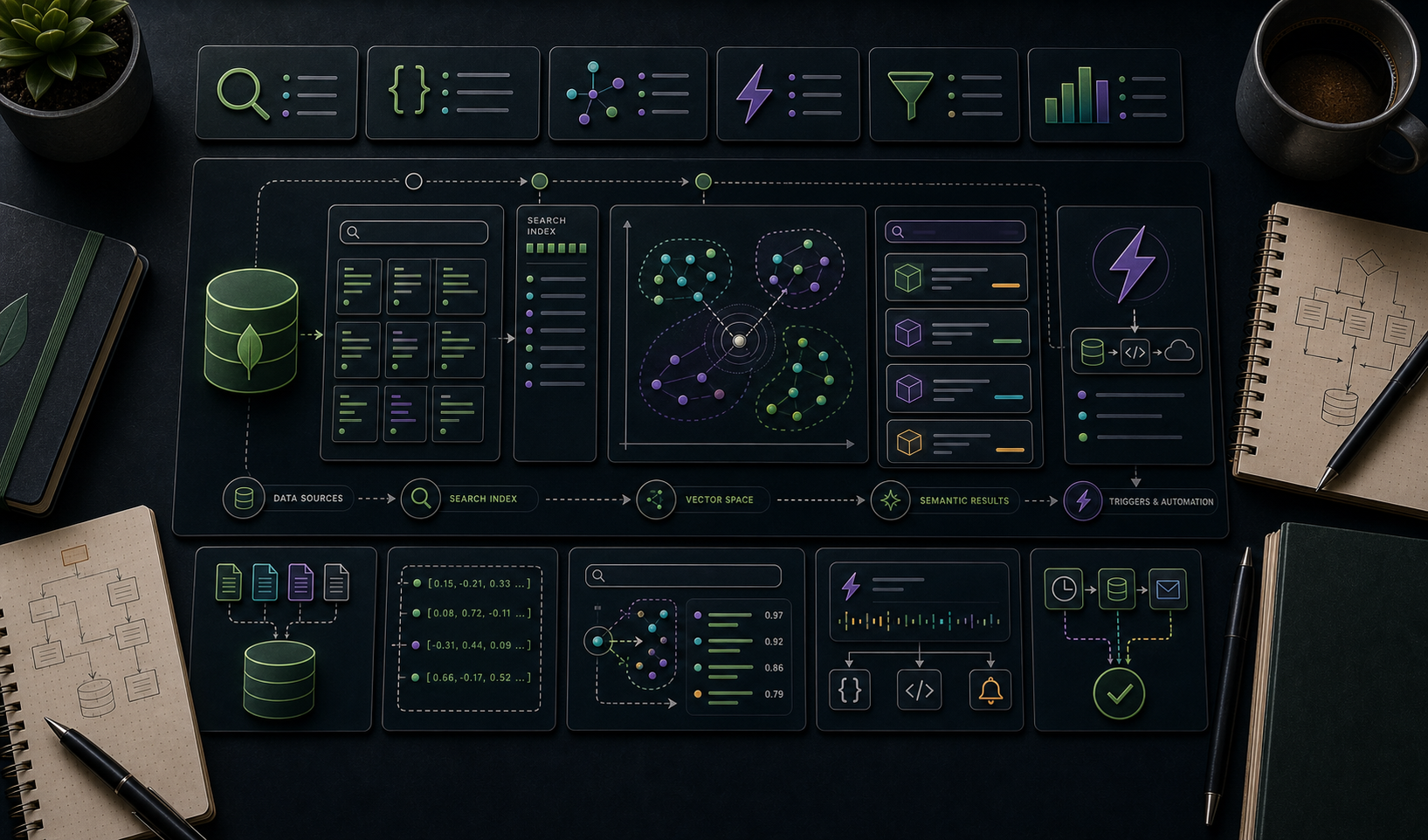
Atlas is MongoDB Inc.'s managed cloud service. Beyond hosting Mongo for you, Atlas ships features the open-source core doesn't have: Atlas Search (Lucene-based full-text), Atlas Vector Search (k-NN over embeddings — the building block of every RAG system in 2026), Atlas Triggers (serverless functions on database events / schedules / HTTP), Atlas Stream Processing (real-time pipelines over Kafka streams + Mongo collections), Atlas Online Archive (tier old data to cheap storage), and Data Federation (one query over Mongo + S3 + more). This post covers all of them with the patterns that show up in production.
> Series map: 00 Foundations → … → 15 Performance Deep → 16 Atlas (this post) → 17 Drivers & Case Studies.
Learning Outcome
- Build an Atlas Search index + run full-text queries with facets, autocomplete, fuzzy.- Build an Atlas Vector Search index + run k-NN over embeddings (RAG basics).- Wire up Atlas Triggers — database / scheduled / HTTP / authentication.- Run an Atlas Stream Processing pipeline over a Kafka source.- Use Online Archive + Data Federation for cost-effective long-term data.
Chapter 1 — Atlas Search (Lucene full-text)
Atlas Search runs a Lucene index alongside your Mongo collection. Updates propagate automatically; queries use the new aggregation stage.
Create the index (UI or since 7.0)
auto-indexes every string field; useful for prototyping, costly at scale.
Search
Compound queries with / / / :
Facets — counts per dimension
Produces counts per facet bucket — perfect for filtered search UIs.
Autocomplete
Add an field type in the index definition ().
Atlas Search replaces (Post 02) for any serious search workload — scoring, autocomplete, fuzzy, facets, multi-language, synonyms.
Chapter 2 — Atlas Vector Search — the RAG building block
Vector Search stores embedding vectors (typically 768-3072 floats) alongside documents and answers k-nearest-neighbour queries. Building block for RAG (Retrieval-Augmented Generation), semantic search, recommendation engines.
Create the index
The index is HNSW (Hierarchical Navigable Small World) under the hood — fast approximate nearest neighbour at scale.
Query
RAG pipeline (end-to-end)
Two Mongo features make this natural:
- One database for the documents + their embeddings + their metadata.- Vector + filter combined (e.g., "semantic search restricted to this tenant's documents only").
Common 2026 embedding choices:
- OpenAI (1536 dim) / (3072 dim).- Cohere (1024 dim).- Open-source on-prem: , , (varies).
Dimension + similarity must match your embedder.
Hybrid search
Combine Atlas Search (lexical) + Vector Search (semantic) for the best of both:
Production RAG systems usually combine both signals + rerank with a small model.
Chapter 3 — Atlas Triggers — serverless events
Triggers run JavaScript / TypeScript functions in response to events. Three trigger types:
Database trigger (change-stream-driven)
Equivalent to running a change-stream consumer yourself (Post 12) but with no infrastructure to manage.
Scheduled trigger (cron)
HTTPS endpoint
Expose your function as an HTTPS API. Standard for lightweight webhooks, integrations.
Authentication trigger
Run on user signup / login / delete in Atlas App Services (Realm) auth.
Triggers are billed per invocation + per millisecond of compute. Free tier covers light workloads. Atlas Functions support npm packages, secrets, HTTPS calls, MongoDB driver built-in.
Chapter 4 — Atlas Stream Processing
Real-time pipelines that combine streams (Kafka) + Atlas collections + sinks (Kafka, collections, S3). Use SQL-like aggregation pipelines over windows of events.
Use cases:
- Real-time aggregation (per-region revenue per 5-minute window).- Stream enrichment (join Kafka clickstream with user profiles in Mongo).- ETL into a warehouse.
Stream Processing is GA in 2026; competes with managed Flink / Kafka Streams. Compelling when your data lives in Atlas anyway.
Chapter 5 — Online Archive
Move old documents to cheap blob storage, queryable via the same connection.
Set up via Atlas UI: pick a collection, define a date-based filter, choose retention. After archive, documents are gone from the primary collection but reachable via the federated database.
Cost: archived data is 10× cheaper than hot tier.
Use cases: compliance retention; lifecycle management; right-sizing the hot cluster.
Chapter 6 — Data Federation
Run one query across Atlas clusters + S3 + other federated sources:
For analytics over years of mixed-tier data, much simpler than ETL + a warehouse.
Chapter 7 — Atlas Charts
A built-in BI tool for visualising MongoDB data. Drag fields, build dashboards, embed via iframe / API. Skips the need for a separate BI tool for small to medium projects.
Pair with -built materialised views (Post 06) for fast dashboard reads.
Chapter 8 — Atlas App Services (formerly Realm)
A serverless backend platform: auth, functions, GraphQL endpoint, HTTPS rules. Pairs naturally with Atlas Triggers + Mongo for full-stack apps without managing servers.
In 2026 the focus shifted toward leaner primitives (Triggers + Functions + HTTPS endpoints) rather than the full Realm stack. Check current docs for the supported feature set.
Chapter 9 — When to lean on Atlas vs DIY
Lean on Atlas when:
- Search + vector + serverless triggers + monitoring are all needed.- Small / medium ops team — managed > self-hosted.- Multi-region HA + automatic backups + PITR are required.- Workloads benefit from one provider (less integration).
DIY (self-hosted Mongo + Elasticsearch + Kafka + cron + S3) when:
- Existing infra investment.- On-prem or sovereign cloud requirement.- Cost optimisation at very large scale.
Most teams below 100-engineer scale benefit from Atlas. Most teams above can justify either way.
Chapter 10 — Cost notes (rough, 2026)
| Resource | Cost driver ||----------|-------------|| Atlas cluster | tier hours (M0 free → M700+ enterprise) || Atlas Search | search node hours + index storage || Atlas Vector Search | same nodes; cost scales with vectors + dims || Triggers / Functions | invocations + compute ms || Stream Processing | processor hours + Kafka egress || Online Archive | storage GB-month + queries || Data Federation | per-GB scanned || Backups | retention storage |
Always check current Atlas pricing page — values shift. Use the Atlas billing dashboard + alerts.
Chapter 11 — Common pitfalls
| Pitfall | Cause | Fix ||---------|-------|-----|| returns 0 — fresh index | indexing in progress | wait + check index status || Vector dim mismatch | model changed; index didn't | rebuild index for new dim || Vector search slow + low recall | too small | raise (cost trade-off) || Trigger silent failure | exception in function | check Atlas Function logs || Stream processor lag | sink slow / window too big | profile sink; smaller windows || Federation query super slow | large S3 scan | partition source data by date / key || Charts dashboard slow | querying raw events | precompute via materialised view || Search costs surprise | dynamic mapping indexing everything | narrow explicitly |
Practice Exercises
Exercise 1 — Search index
On a sample collection, create an Atlas Search index. Query for "mongodb" with fuzzy + autocomplete.
Exercise 2 — Vector search RAG
Generate embeddings (OpenAI / Cohere / local model) for a handful of documents. Store in Mongo. Build a vector index. Run k-NN for a user query embedding. Confirm relevant docs returned.
Exercise 3 — Trigger on insert
Write an Atlas Database trigger on that posts a webhook with the new order. Test by inserting; confirm webhook receives the payload.
Exercise 4 — Scheduled refresh
Build a scheduled trigger that refreshes via every hour.
Exercise 5 — Hybrid search
Combine lexical search + vector search with (Chapter 2). Compare top 10 results vs lexical-only vs vector-only.
Exercise 6 — Online Archive
Set up archive on a synthetic collection — move data > 30 days old. Query via federation across hot + archive; confirm transparency.
Cheat-sheet
| What | How ||------|-----|| Search index | UI or || Text search | || Compound | || Facets | || Autocomplete | field type + || Vector index | , fields: + filter || Vector query | || Similarity | cosine / euclidean / dotProduct || RAG pipeline | embed → store → query embed → $vectorSearch → LLM prompt || Hybrid | + + + rerank || Database trigger | runs on change events || Scheduled trigger | cron form || HTTPS endpoint | trigger + URL || Stream Processing | → → || Online Archive | tier old data to cheap storage; still queryable || Data Federation | one query across many sources || Charts | built-in dashboards || When Atlas | small/mid teams; broad managed feature need |
What's next
Post 17 — the final base post — covers drivers + modelling case studies: Node official + Mongoose vs Prisma, Python pymongo + Motor, Go, Rust, and end-to-end models for time-series, IoT telemetry, e-commerce catalogue, social feed, multi-tenant SaaS.
References
- Atlas Search- Atlas Vector Search- Atlas Triggers- Atlas Stream Processing- Online Archive- Data Federation
> Note: this post is in progress. Planned additions: end-to-end RAG sample app (Next.js + OpenAI + Atlas Vector); benchmark of HNSW recall vs ; cost case studies.
Linear Algebra — 02 · Vector Spaces, Subspaces, Basis and Dimension
Linear Algebra 00 and 01 worked with columns of numbers. This post asks what those columns have in common with polynomials, functions, matrices and the solutions of a differential equation — and answers with one definition: a vector space. From that definition come the ideas that organise the rest of the subject: subspaces, span, linear independence, basis and dimension. The central theorem is that dimension is well defined — every basis of a space has the same size — and it is proved here in full through the Steinitz exchange lemma. The abstract ideas are then brought back to matrices through Strang's four fundamental subspaces, with a complete worked example, a proof that row rank equals column rank, and the rank–nullity theorem in matrix form. The post ends with sums and direct sums of subspaces and the formula $\dim(U + W) = \dim U + \dim W - \dim(U \cap W)$.
> Series map: 00 Vectors & Linear Systems → 01 Matrix Algebra, Inverses & LU → 02 Vector Spaces, Basis & Dimension (this post) → 03 Linear Maps, Change of Basis & Determinants → 04 Eigenvalues & Diagonalization → 05 Inner Products, Spectral Theorem & SVD.
Learning Outcome
- State the axioms of a vector space over a field, and check them for $F^n$, polynomials, functions and matrices.- Prove simple consequences of the axioms, such as $0\mathbf{v} = \mathbf{0}$ and $(-1)\mathbf{v} = -\mathbf{v}$.- Use the subspace test, and recognise common subspaces and non-subspaces.- Work with span and linear independence in any vector space, including the linear dependence lemma.- Prove the Steinitz exchange lemma and deduce that dimension is well defined.- Extend an independent list to a basis, shrink a spanning list to a basis, and compute coordinates.- Find bases and dimensions of the four fundamental subspaces of a matrix from its RREF.- Prove that row rank equals column rank and that $\operatorname{rank} A + \dim N(A) = n$.- Work with sums and direct sums, and prove the dimension formula for $U + W$.
Chapter 1 — Fields and vector spaces
Terminology
- Field — a set $F$ with an addition and a multiplication that satisfy the usual rules of arithmetic: both operations are associative and commutative, multiplication distributes over addition, there are elements $0 \neq 1$ with $a + 0 = a$ and $1a = a$, every $a$ has a negative $-a$, and every nonzero $a$ has an inverse $a^{-1}$. Examples: $\mathbb{Q}$, $\mathbb{R}$, $\mathbb{C}$, and $\mathbb{F}2 = \{0, 1\}$ with arithmetic mod 2. The integers $\mathbb{Z}$ are not a field ($2$ has no integer inverse).- Scalars — the elements of the field. In this series $F$ is $\mathbb{R}$ or $\mathbb{C}$ unless stated.
Everything in Linear Algebra 00 and 01 — elimination, pivots, inverses, LU — used only these field rules, so it works word for word over any field.
The definition
A vector space over $F$ is a set $V$ with an addition $V \times V \to V$ and a scalar multiplication $F \times V \to V$ such that, for all $\mathbf{u}, \mathbf{v}, \mathbf{w} \in V$ and $a, b \in F$:
1. $\mathbf{u} + \mathbf{v} = \mathbf{v} + \mathbf{u}$ (commutativity).2. $(\mathbf{u} + \mathbf{v}) + \mathbf{w} = \mathbf{u} + (\mathbf{v} + \mathbf{w})$ (associativity).3. There is an element $\mathbf{0} \in V$ with $\mathbf{v} + \mathbf{0} = \mathbf{v}$ for all $\mathbf{v}$ (additive identity).4. For each $\mathbf{v}$ there is $\mathbf{w}$ with $\mathbf{v} + \mathbf{w} = \mathbf{0}$ (additive inverse).5. $a(b\mathbf{v}) = (ab)\mathbf{v}$.6. $1\mathbf{v} = \mathbf{v}$.7. $a(\mathbf{u} + \mathbf{v}) = a\mathbf{u} + a\mathbf{v}$.8. $(a + b)\mathbf{v} = a\mathbf{v} + b\mathbf{v}$.
The elements of $V$ are called vectors, whatever they actually are.
First consequences
Proposition. In any vector space: (a) the zero vector is unique; (b) each $\mathbf{v}$ has exactly one additive inverse, written $-\mathbf{v}$; (c) $0\mathbf{v} = \mathbf{0}$; (d) $a\mathbf{0} = \mathbf{0}$; (e) $(-1)\mathbf{v} = -\mathbf{v}$.
Proof. (a) If $\mathbf{0}$ and $\mathbf{0}'$ are both identities, $\mathbf{0} = \mathbf{0} + \mathbf{0}' = \mathbf{0}'$. (b) If $\mathbf{w}, \mathbf{w}'$ are both inverses of $\mathbf{v}$, then $\mathbf{w} = \mathbf{w} + (\mathbf{v} + \mathbf{w}') = (\mathbf{w} + \mathbf{v}) + \mathbf{w}' = \mathbf{w}'$. (c) $0\mathbf{v} = (0 + 0)\mathbf{v} = 0\mathbf{v} + 0\mathbf{v}$; add $-(0\mathbf{v})$ to both sides. (d) The same with $a\mathbf{0} = a(\mathbf{0} + \mathbf{0})$. (e) $\mathbf{v} + (-1)\mathbf{v} = (1 + (-1))\mathbf{v} = 0\mathbf{v} = \mathbf{0}$, so $(-1)\mathbf{v}$ is the inverse of $\mathbf{v}$, by (b). $\blacksquare$
Examples
| Space | Vectors | Operations ||---|---|---|| $F^n$ | columns $(x1, \dots, xn)$ | entry by entry || $\mathcal{P}n(F)$ | polynomials of degree at most $n$ | add coefficients; scale coefficients || $\mathcal{P}(F)$ | all polynomials | same || $F^S$ | all functions $f : S \to F$ on a set $S$ | $(f + g)(s) = f(s) + g(s)$, $(af)(s) = a f(s)$ || $C[a, b]$ | continuous real functions on $[a, b]$ | pointwise || $M{m \times n}(F)$ | $m \times n$ matrices | entry by entry |
$F^n$ is really the special case $F^S$ with $S = \{1, \dots, n\}$: a column is a function from positions to numbers.
Non-examples. The first quadrant $\{(x, y) : x, y \ge 0\}$ fails axiom 4 — $(1, 0)$ has no inverse inside it. The line $\{(x, y) : y = x + 1\}$ has no zero vector. The polynomials of degree exactly 2 are not closed under addition: $(t^2 + t) + (-t^2) = t$.
Chapter 2 — Subspaces
Terminology
- Subspace — a subset $U \subseteq V$ that is itself a vector space with the same addition and scalar multiplication.
Theorem (subspace test). A subset $U$ of a vector space $V$ is a subspace if and only if
1. $\mathbf{0} \in U$;2. $\mathbf{u}, \mathbf{w} \in U \Rightarrow \mathbf{u} + \mathbf{w} \in U$ (closed under addition);3. $a \in F$, $\mathbf{u} \in U \Rightarrow a\mathbf{u} \in U$ (closed under scalar multiplication).
Proof. A subspace clearly satisfies 2 and 3, and it contains its own zero vector $\mathbf{z}$ with $\mathbf{z} + \mathbf{z} = \mathbf{z}$; adding $-\mathbf{z}$ in $V$ shows $\mathbf{z} = \mathbf{0}$, so 1 holds. Conversely, suppose 1–3 hold. Conditions 2 and 3 make addition and scalar multiplication land in $U$. Axioms 1, 2, 5–8 are identities that hold for all vectors of $V$, so in particular for those of $U$. Axiom 3 holds by condition 1. For axiom 4: if $\mathbf{u} \in U$ then $-\mathbf{u} = (-1)\mathbf{u} \in U$ by condition 3 and part (e) of the proposition. $\blacksquare$
> Trick: conditions 2 and 3 together are the same as "closed under linear combinations": $a\mathbf{u} + b\mathbf{w} \in U$ for all $\mathbf{u}, \mathbf{w} \in U$ and scalars $a, b$. Check $\mathbf{0}$ first — it is the fastest way to reject a non-subspace.
Examples and non-examples
- Null space $N(A) = \{\mathbf{x} \in F^n : A\mathbf{x} = \mathbf{0}\}$ is a subspace of $F^n$: $A\mathbf{0} = \mathbf{0}$, and $A(a\mathbf{u} + b\mathbf{w}) = aA\mathbf{u} + bA\mathbf{w} = \mathbf{0}$.- Column space $C(A) = \{A\mathbf{x} : \mathbf{x} \in F^n\}$, the span of the columns, is a subspace of $F^m$.- $\{p \in \mathcal{P}2(\mathbb{R}) : p(1) = 0\}$ is a subspace; $\{p : p(1) = 5\}$ is not (no zero polynomial).- The symmetric $n \times n$ matrices form a subspace of $M{n \times n}$.- The solutions $y$ of $y'' + y = 0$ form a subspace of the twice-differentiable functions $\mathbb{R} \to \mathbb{R}$.- The solutions of $A\mathbf{x} = \mathbf{b}$ with $\mathbf{b} \neq \mathbf{0}$ are not a subspace (Linear Algebra 00, Chapter 7): $\mathbf{0}$ is not a solution.- The union of the $x$-axis and the $y$-axis in $\mathbb{R}^2$ is not a subspace: $(1, 0) + (0, 1) = (1, 1)$ is in neither.
Intersections are subspaces. If $U$ and $W$ are subspaces, so is $U \cap W$: it contains $\mathbf{0}$, and a linear combination of vectors in both lies in both. Unions usually are not, as the axes show; Chapter 8 replaces the union by the sum $U + W$.
Chapter 3 — Span and linear independence in general
The definitions from Linear Algebra 00 carry over unchanged. For a finite list $\mathbf{v}1, \dots, \mathbf{v}k$ in $V$:
- $\operatorname{span}(\mathbf{v}1, \dots, \mathbf{v}k)$ is the set of all linear combinations $a1\mathbf{v}1 + \dots + ak\mathbf{v}k$. By convention the span of the empty list is $\{\mathbf{0}\}$.- The list spans $V$ if its span is all of $V$.- The list is linearly independent if $a1\mathbf{v}1 + \dots + ak\mathbf{v}k = \mathbf{0}$ forces $a1 = \dots = ak = 0$; otherwise it is dependent. The empty list is independent.
Proposition. $\operatorname{span}(\mathbf{v}1, \dots, \mathbf{v}k)$ is the smallest subspace of $V$ containing every $\mathbf{v}i$.
Proof. It contains $\mathbf{0}$, and a combination of combinations is a combination, so it is a subspace; it contains each $\mathbf{v}i$. Any subspace containing all $\mathbf{v}i$ is closed under linear combinations, so it contains the span. $\blacksquare$
The linear dependence lemma
Lemma. If $\mathbf{v}1, \dots, \mathbf{v}m$ is linearly dependent, then there is an index $j$ such that
1. $\mathbf{v}j \in \operatorname{span}(\mathbf{v}1, \dots, \mathbf{v}{j-1})$, and2. removing $\mathbf{v}j$ from the list does not change its span.
Proof. Take a relation $a1\mathbf{v}1 + \dots + am\mathbf{v}m = \mathbf{0}$ with not all $ai = 0$, and let $j$ be the largest index with $aj \neq 0$. Then
$$\mathbf{v}j = -\frac{a1}{aj}\mathbf{v}1 - \dots - \frac{a{j-1}}{aj}\mathbf{v}{j-1},$$
which proves 1. (If $j = 1$ this says $\mathbf{v}1 = \mathbf{0}$, the span of the empty list.) For 2, in any combination of the full list, replace $\mathbf{v}j$ by the right-hand side above; the result is a combination of the list without $\mathbf{v}j$. $\blacksquare$
Independence outside Fⁿ
- In $\mathcal{P}2(\mathbb{R})$, the list $1, t, t^2$ is independent: if $a + bt + ct^2$ is the zero polynomial, all its coefficients are 0.- In the functions $\mathbb{R} \to \mathbb{R}$, $\sin$ and $\cos$ are independent: if $a\sin x + b\cos x = 0$ for all $x$, then $x = 0$ gives $b = 0$ and $x = \pi/2$ gives $a = 0$.
> Common pitfall: "$a\sin x + b\cos x = 0$" means equality as functions, for every $x$. Finding one $x$ where a combination is zero proves nothing; you must show the combination is zero everywhere only when all weights are zero.
Chapter 4 — Basis, the exchange lemma and dimension
Terminology
- Basis of $V$ — a list of vectors in $V$ that is linearly independent and spans $V$.- Finite-dimensional — $V$ is spanned by some finite list. Otherwise infinite-dimensional.- Standard basis of $F^n$ — $\mathbf{e}1, \dots, \mathbf{e}n$. Of $\mathcal{P}n(F)$ — $1, t, \dots, t^n$.
Theorem (unique representation). A list $\mathbf{v}1, \dots, \mathbf{v}n$ is a basis of $V$ if and only if every $\mathbf{v} \in V$ can be written as $a1\mathbf{v}1 + \dots + an\mathbf{v}n$ in exactly one way.
Proof. Spanning is "at least one way". If a basis gave two ways, subtracting them gives $\sum (ai - bi)\mathbf{v}i = \mathbf{0}$, so every $ai = bi$ by independence. Conversely, uniqueness for $\mathbf{v} = \mathbf{0}$ (which is $0\mathbf{v}1 + \dots + 0\mathbf{v}n$) is exactly independence. $\blacksquare$
The Steinitz exchange lemma
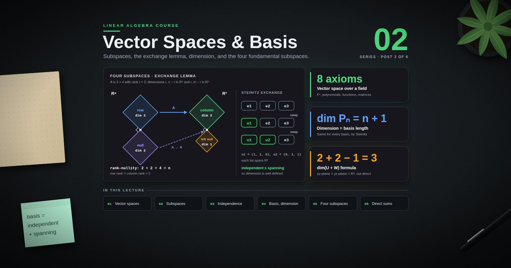
Lemma (Steinitz exchange). Let $V$ be a vector space. Suppose $\mathbf{u}1, \dots, \mathbf{u}m$ is linearly independent in $V$ and $\mathbf{w}1, \dots, \mathbf{w}n$ spans $V$. Then $m \le n$. Moreover, after renumbering the $\mathbf{w}$'s, the list
$$\mathbf{u}1, \dots, \mathbf{u}m, \mathbf{w}{m+1}, \dots, \mathbf{w}n$$
also spans $V$.
Proof. We show by induction on $k = 0, 1, \dots, m$ that $k \le n$ and that, after renumbering, $\mathbf{u}1, \dots, \mathbf{u}k, \mathbf{w}{k+1}, \dots, \mathbf{w}n$ spans $V$. For $k = 0$ this is the hypothesis.
Assume it holds for some $k < m$. Since the list $\mathbf{u}1, \dots, \mathbf{u}k, \mathbf{w}{k+1}, \dots, \mathbf{w}n$ spans $V$, we can write
$$\mathbf{u}{k+1} = a1\mathbf{u}1 + \dots + ak\mathbf{u}k + b{k+1}\mathbf{w}{k+1} + \dots + bn\mathbf{w}n.$$
If every $bj$ were 0 (in particular, if no $\mathbf{w}$'s were left, $k = n$), then $\mathbf{u}{k+1}$ would be a combination of $\mathbf{u}1, \dots, \mathbf{u}k$, contradicting independence of the $\mathbf{u}$'s. So some $bj \neq 0$; hence $k + 1 \le n$. Renumber so that $b{k+1} \neq 0$ and solve for $\mathbf{w}{k+1}$:
$$\mathbf{w}{k+1} = \frac{1}{b{k+1}}\Bigl(\mathbf{u}{k+1} - \sum{i=1}^{k} ai\mathbf{u}i - \sum{j=k+2}^{n} bj\mathbf{w}j\Bigr).$$
So $\mathbf{w}{k+1}$ lies in the span of $\mathbf{u}1, \dots, \mathbf{u}{k+1}, \mathbf{w}{k+2}, \dots, \mathbf{w}n$. That span therefore contains the whole old spanning list, so it is $V$. This completes the step. At $k = m$ we get $m \le n$ and the stated spanning list. $\blacksquare$
Small example. In $\mathbb{R}^3$ take the independent $\mathbf{u}1 = (1, 1, 0)$, $\mathbf{u}2 = (0, 1, 1)$ and the spanning $\mathbf{e}1, \mathbf{e}2, \mathbf{e}3$. Since $\mathbf{u}1 = \mathbf{e}1 + \mathbf{e}2$ has a nonzero coefficient on $\mathbf{e}1$, swap it out: $\mathbf{u}1, \mathbf{e}2, \mathbf{e}3$ spans. Then $\mathbf{u}2 = 0\,\mathbf{u}1 + \mathbf{e}2 + \mathbf{e}3$; swap out $\mathbf{e}2$: $\mathbf{u}1, \mathbf{u}2, \mathbf{e}3$ spans $\mathbb{R}^3$. (Three vectors that span $\mathbb{R}^3$ are automatically a basis — see the theorem at the end of this chapter.)
Dimension is well defined
Theorem. In a finite-dimensional vector space, any two bases have the same length.
Proof. Let $B1$ and $B2$ be bases, of lengths $m$ and $n$. $B1$ is independent and $B2$ spans, so $m \le n$ by Steinitz. Swap roles: $n \le m$. $\blacksquare$
This common length is the dimension $\dim V$.
| Space | Dimension | A basis ||---|---|---|| $\{\mathbf{0}\}$ | 0 | the empty list || $F^n$ | $n$ | $\mathbf{e}1, \dots, \mathbf{e}n$ || $\mathcal{P}n(F)$ | $n + 1$ | $1, t, \dots, t^n$ || $M{m \times n}(F)$ | $mn$ | matrices with one entry 1, the rest 0 || symmetric $2 \times 2$ | 3 | one basis matrix each for the (1,1), (2,2) and paired off-diagonal entries || $\mathcal{P}(F)$ | infinite | $1, t, t^2, \dots$ (no finite list spans) |
> Watch out: $\mathbb{C}^n$ has dimension $n$ over $\mathbb{C}$ but $2n$ over $\mathbb{R}$ (a basis over $\mathbb{R}$ is $\mathbf{e}1, i\mathbf{e}1, \dots, \mathbf{e}n, i\mathbf{e}n$). Dimension depends on the field of scalars.
Growing and shrinking to a basis
Theorem. Let $V$ be finite-dimensional with $\dim V = n$.
1. Every spanning list can be shrunk to a basis by removing vectors.2. Every independent list can be extended to a basis by adding vectors.3. Any $n$ independent vectors form a basis; any $n$ spanning vectors form a basis.4. Every subspace $U$ is finite-dimensional with $\dim U \le n$, and $\dim U = n$ only if $U = V$.
Proof. (1) While the list is dependent, the dependence lemma lets you remove one vector without changing the span. The process stops at an independent spanning list. (2) Apply Steinitz with a basis as the spanning list: the independent list plus the remaining $n - m$ basis vectors spans $V$; it has length $n$, and by (1) some sublist is a basis, which must have length $n$, so it is the whole list. (3) An independent list of length $n$ extends to a basis of length $n$, so nothing is added; a spanning list of length $n$ shrinks to a basis of length $n$, so nothing is removed. (4) Any independent list in $U$ is independent in $V$, so it has length at most $n$ by Steinitz. Keep adding vectors of $U$ not yet in the span of an independent list (independence is kept, by Exercise 7); this stops after at most $n$ steps with a basis of $U$. If $\dim U = n$, that basis is $n$ independent vectors of $V$, so by (3) it spans $V$, hence $U = V$. $\blacksquare$
Chapter 5 — Coordinates
If $B = (\mathbf{v}1, \dots, \mathbf{v}n)$ is a basis of $V$, each $\mathbf{v}$ has unique weights with $\mathbf{v} = a1\mathbf{v}1 + \dots + an\mathbf{v}n$. The column $[\mathbf{v}]B = (a1, \dots, an) \in F^n$ is the coordinate vector of $\mathbf{v}$ relative to $B$.
The map $\mathbf{v} \mapsto [\mathbf{v}]B$ is one-to-one, onto $F^n$, and respects linear combinations: $[a\mathbf{u} + b\mathbf{w}]B = a[\mathbf{u}]B + b[\mathbf{w}]B$. So every $n$-dimensional space over $F$ behaves exactly like $F^n$, and computations in it can be done with columns and matrices. Linear Algebra 03 makes this precise (isomorphism) and studies how coordinates change when the basis changes.
Example in $\mathbb{R}^2$. With $B = ((1, 1), (1, -1))$ and $\mathbf{x} = (3, 1)$: solve $a(1,1) + b(1,-1) = (3, 1)$, so $a + b = 3$, $a - b = 1$, giving $a = 2$, $b = 1$. So $[\mathbf{x}]B = (2, 1)$, while the standard coordinates are $(3, 1)$ — same vector, different description.
Example in $\mathcal{P}2(\mathbb{R})$. With $B = (1,\ 1 + t,\ (1 + t)^2)$, find $[t^2]B$. Put $s = 1 + t$; then $t = s - 1$ and $t^2 = s^2 - 2s + 1$. So
$$t^2 = 1 \cdot (1 + t)^2 - 2(1 + t) + 1 \cdot 1, \qquad [t^2]B = (1, -2, 1)$$
(the weights on $1$, $1 + t$ and $(1 + t)^2$, in that order). Check: $(1 + 2t + t^2) - 2 - 2t + 1 = t^2$.
Chapter 6 — The four fundamental subspaces
Terminology
For an $m \times n$ matrix $A$ of rank $r$ (the number of pivots):
| Subspace | Symbol | Lives in | Definition ||---|---|---|---|| Column space | $C(A)$ | $F^m$ | all $A\mathbf{x}$; span of the columns || Null space | $N(A)$ | $F^n$ | all $\mathbf{x}$ with $A\mathbf{x} = \mathbf{0}$ || Row space | $C(A^T)$ | $F^n$ | span of the rows || Left null space | $N(A^T)$ | $F^m$ | all $\mathbf{y}$ with $A^T\mathbf{y} = \mathbf{0}$, that is $\mathbf{y}^TA = \mathbf{0}^T$ |
Two facts about row operations
Let $EA = R$ with $E$ invertible (a product of elementary matrices) and $R$ the RREF.
Fact 1 — the row space does not change. Every row of $R$ is a combination of rows of $A$, and since $A = E^{-1}R$, every row of $A$ is a combination of rows of $R$. So $C(A^T) = C(R^T)$.
Fact 2 — linear relations among columns do not change. $A\mathbf{x} = \mathbf{0} \iff EA\mathbf{x} = \mathbf{0} \iff R\mathbf{x} = \mathbf{0}$, because $E$ is invertible. So a combination of columns of $A$ is zero exactly when the same combination of columns of $R$ is zero, and $N(A) = N(R)$. (The column spaces of $A$ and $R$ usually differ.)
Bases from the RREF
- $C(A)$ — the pivot columns of $A$ (not of $R$). In $R$ the pivot columns are distinct standard basis vectors, so they are independent, and every other column is a combination of them. By Fact 2 the same holds for the corresponding columns of $A$.- $C(A^T)$ — the nonzero rows of $R$. They span the row space by Fact 1, and they are independent because each has a leading 1 in a column where the other rows have 0.- $N(A)$ — the $n - r$ special solutions (one free variable 1, the others 0), as in Linear Algebra 00.- $N(A^T)$ — the last $m - r$ rows of $E$: those rows multiply $A$ to give the zero rows of $R$.
Worked example
Use the matrix from Linear Algebra 00, Chapter 6:
$$A = \begin{pmatrix} 1 & 2 & 2 & 2 \\ 2 & 4 & 6 & 8 \\ 3 & 6 & 8 & 10 \end{pmatrix}, \qquadR = \begin{pmatrix} 1 & 2 & 0 & -2 \\ 0 & 0 & 1 & 2 \\ 0 & 0 & 0 & 0 \end{pmatrix}, \qquad m = 3,\ n = 4,\ r = 2.$$
Pivot columns 1 and 3; free variables $x2, x4$.
- Column space (dimension $r = 2$, in $\mathbb{R}^3$): basis $(1, 2, 3)$ and $(2, 6, 8)$ — columns 1 and 3 of $A$. The other columns satisfy the same relations as in $R$: column 2 $= 2 \times$ column 1, and column 4 $= -2 \times$ column 1 $+ 2 \times$ column 3. Check: $-2(1,2,3) + 2(2,6,8) = (2, 8, 10)$.- Row space (dimension $r = 2$, in $\mathbb{R}^4$): basis $(1, 2, 0, -2)$ and $(0, 0, 1, 2)$.- Null space (dimension $n - r = 2$, in $\mathbb{R}^4$): basis $\mathbf{s}1 = (-2, 1, 0, 0)$ and $\mathbf{s}2 = (2, 0, -2, 1)$.- Left null space (dimension $m - r = 1$, in $\mathbb{R}^3$): the elimination steps $R2 - 2R1$, $R3 - 3R1$, $R3 - R2$ make row 3 into $-(\text{row } 1) - (\text{row } 2) + (\text{row } 3) = \mathbf{0}$. So $\mathbf{y} = (-1, -1, 1)$ is a basis: $\mathbf{y}^TA = \mathbf{0}^T$.
Orthogonality — a preview
Each row of $A$ dotted with a null-space vector gives 0 — that is what $A\mathbf{x} = \mathbf{0}$ says, one row at a time. So every vector of $N(A)$ is orthogonal to every vector of $C(A^T)$. In the example, $(1, 2, 0, -2)\cdot(-2, 1, 0, 0) = 0$, $(1, 2, 0, -2)\cdot(2, 0, -2, 1) = 0$, $(0, 0, 1, 2)\cdot(-2, 1, 0, 0) = 0$ and $(0, 0, 1, 2)\cdot(2, 0, -2, 1) = 0$. In the same way $N(A^T)$ is orthogonal to $C(A)$: $(-1, -1, 1)\cdot(1, 2, 3) = 0$ and $(-1, -1, 1)\cdot(2, 6, 8) = 0$. Over $\mathbb{R}$ the dimensions add up ($2 + 2 = 4$, $2 + 1 = 3$), which makes each pair orthogonal complements — proved in Linear Algebra 05.
Row rank equals column rank
Theorem. For every matrix, $\dim C(A) = \dim C(A^T) = r$, the number of pivots.
Proof. The pivot columns of $A$ are a basis of $C(A)$, and there are $r$ of them. The nonzero rows of $R$ are a basis of $C(A^T)$, and there are $r$ of them (one per pivot). $\blacksquare$
This is not obvious: for a $3 \times 100$ matrix it says that the 100 columns span a space of the same dimension as the 3 rows. It also shows $\operatorname{rank} A = \operatorname{rank} A^T$, and that $r \le \min(m, n)$.
Rank-one matrices. A matrix has rank 1 exactly when it is a nonzero column times a nonzero row, $A = \mathbf{u}\mathbf{v}^T$: every column is a multiple of $\mathbf{u}$, every row a multiple of $\mathbf{v}^T$. The outer-product view of Linear Algebra 01 writes any $AB$ as a sum of such pieces.
Chapter 7 — Rank–nullity (matrix form)
Theorem (rank–nullity). For an $m \times n$ matrix $A$,
$$\dim C(A) + \dim N(A) = n.$$
Proof. Let $r$ be the number of pivots. $\dim C(A) = r$ by Chapter 6. It remains to show that the $n - r$ special solutions $\mathbf{s}1, \dots, \mathbf{s}{n-r}$ are a basis of $N(A)$.
Independent: look only at the free-variable entries. In $\mathbf{s}k$ the $k$-th free variable is 1 and the others are 0. So in $\sum ck\mathbf{s}k$ the $k$-th free entry is $ck$; if the sum is $\mathbf{0}$, every $ck = 0$.
Spanning: let $\mathbf{x} \in N(A)$ with free-variable values $f1, \dots, f{n-r}$. Then $\mathbf{z} = \mathbf{x} - \sum fk\mathbf{s}k$ is in $N(A)$ and has every free variable equal to 0. The RREF expresses each basic variable in terms of the free ones, so all basic variables of $\mathbf{z}$ are 0 too; thus $\mathbf{z} = \mathbf{0}$ and $\mathbf{x} = \sum fk\mathbf{s}k$.
So $\dim N(A) = n - r$, and $r + (n - r) = n$. $\blacksquare$
In words: each of the $n$ columns either contributes a pivot (a new direction in the column space) or a free variable (a new direction in the null space). For the example, $2 + 2 = 4$. Applied to $A^T$ (which has $m$ columns and the same rank), it gives $\dim N(A^T) = m - r$, here $3 - 2 = 1$.
The general version — for a linear map $T : V \to W$, $\dim V = \dim \operatorname{im} T + \dim \ker T$ — is proved in Linear Algebra 03.
Consequences
| Condition on the rank | Meaning for $A\mathbf{x} = \mathbf{b}$ ||---|---|| $r = m$ (full row rank) | solvable for every $\mathbf{b}$; $C(A) = F^m$ || $r = n$ (full column rank) | at most one solution; $N(A) = \{\mathbf{0}\}$ || $r = m = n$ | exactly one solution; $A$ invertible || $r < m$ and $r < n$ | either no solution or infinitely many |
For a square matrix, "rank $n$", "$N(A) = \{\mathbf{0}\}$" and "$C(A) = F^n$" join the invertible matrix theorem from Linear Algebra 01.
> Trick: rank–nullity is a quick sanity check. A $5 \times 7$ matrix has rank at most 5, so its null space has dimension at least $7 - 5 = 2$ — there are nonzero solutions of $A\mathbf{x} = \mathbf{0}$ before any computation.
Chapter 8 — Sums and direct sums
Terminology
- Sum of subspaces $U, W \subseteq V$: $U + W = \{\mathbf{u} + \mathbf{w} : \mathbf{u} \in U, \mathbf{w} \in W\}$. It is the smallest subspace containing both (a subspace containing $U$ and $W$ contains all such sums).- Direct sum — the sum is direct, written $U \oplus W$, if every vector of $U + W$ can be written as $\mathbf{u} + \mathbf{w}$ in only one way.
Proposition. $U + W$ is direct if and only if $U \cap W = \{\mathbf{0}\}$.
Proof. Suppose the sum is direct and $\mathbf{v} \in U \cap W$. Then $\mathbf{0} = \mathbf{v} + (-\mathbf{v})$ with $\mathbf{v} \in U$, $-\mathbf{v} \in W$, and also $\mathbf{0} = \mathbf{0} + \mathbf{0}$; uniqueness gives $\mathbf{v} = \mathbf{0}$. Conversely, if $U \cap W = \{\mathbf{0}\}$ and $\mathbf{u} + \mathbf{w} = \mathbf{u}' + \mathbf{w}'$, then $\mathbf{u} - \mathbf{u}' = \mathbf{w}' - \mathbf{w}$ lies in both $U$ and $W$, so it is $\mathbf{0}$. $\blacksquare$
> Watch out: for three or more subspaces, pairwise zero intersections are not enough. Three distinct lines through the origin in $\mathbb{R}^2$ meet pairwise only at $\mathbf{0}$, but their sum is not direct (three vectors in $\mathbb{R}^2$ are dependent).
The dimension formula
Theorem. If $U$ and $W$ are finite-dimensional subspaces of $V$, then
$$\dim(U + W) = \dim U + \dim W - \dim(U \cap W).$$
Proof. Let $\mathbf{z}1, \dots, \mathbf{z}k$ be a basis of $U \cap W$. Extend it to a basis $\mathbf{z}1, \dots, \mathbf{z}k, \mathbf{u}1, \dots, \mathbf{u}p$ of $U$ and to a basis $\mathbf{z}1, \dots, \mathbf{z}k, \mathbf{w}1, \dots, \mathbf{w}q$ of $W$ (Chapter 4). The combined list $\mathbf{z}1, \dots, \mathbf{z}k, \mathbf{u}1, \dots, \mathbf{u}p, \mathbf{w}1, \dots, \mathbf{w}q$ clearly spans $U + W$. For independence, suppose
$$\sum ai\mathbf{z}i + \sum bj\mathbf{u}j + \sum cl\mathbf{w}l = \mathbf{0}.$$
Then $\sum cl\mathbf{w}l = -\sum ai\mathbf{z}i - \sum bj\mathbf{u}j$ lies in $W$ and in $U$, hence in $U \cap W$, so $\sum cl\mathbf{w}l = \sum di\mathbf{z}i$ for some $di$. The $\mathbf{z}$'s and $\mathbf{w}$'s together are a basis of $W$, so all $cl = 0$ (and all $di = 0$). Now $\sum ai\mathbf{z}i + \sum bj\mathbf{u}j = \mathbf{0}$ is a relation in a basis of $U$, so all $ai, bj = 0$. Hence the combined list is a basis, and
$$\dim(U + W) = k + p + q = (k + p) + (k + q) - k. \qquad \blacksquare$$
This is the same shape as $\lvert A \cup B\rvert = \lvert A\rvert + \lvert B\rvert - \lvert A \cap B\rvert$ for finite sets.
Examples
- In $\mathbb{R}^3$, let $U = \operatorname{span}(\mathbf{e}1, \mathbf{e}2)$ (the $xy$-plane) and $W = \operatorname{span}(\mathbf{e}2, \mathbf{e}3)$ (the $yz$-plane). Then $U \cap W = \operatorname{span}(\mathbf{e}2)$ and $\dim(U + W) = 2 + 2 - 1 = 3$, so $U + W = \mathbb{R}^3$, but the sum is not direct.- The plane $P = \{\mathbf{x} : x1 + x2 + x3 = 0\}$ and the line $L = \operatorname{span}(1, 1, 1)$ satisfy $P \cap L = \{\mathbf{0}\}$ (a point $(c, c, c)$ with $3c = 0$), so $\dim(P + L) = 2 + 1 = 3$ and $\mathbb{R}^3 = P \oplus L$. For example $(1, 2, 3) = (-1, 0, 1) + (2, 2, 2)$.- Every square matrix splits uniquely into symmetric plus skew-symmetric parts, $M = \tfrac12(M + M^T) + \tfrac12(M - M^T)$, so over $\mathbb{R}$ or $\mathbb{C}$ (any field where $2 \neq 0$), $M{n \times n} = \text{Sym} \oplus \text{Skew}$. For $M = \begin{pmatrix} 1 & 2 \\ 4 & 3 \end{pmatrix}$ the parts are $\begin{pmatrix} 1 & 3 \\ 3 & 3 \end{pmatrix}$ and $\begin{pmatrix} 0 & -1 \\ 1 & 0 \end{pmatrix}$.- For a real $m \times n$ matrix, $\mathbb{R}^n = C(A^T) \oplus N(A)$. The intersection is $\{\mathbf{0}\}$, because a vector in both is orthogonal to itself, and $\mathbf{x}\cdot\mathbf{x} = 0$ forces $\mathbf{x} = \mathbf{0}$; the dimensions add to $r + (n - r) = n$. So every $\mathbf{x} \in \mathbb{R}^n$ splits uniquely as $\mathbf{x} = \mathbf{x}r + \mathbf{x}n$, a row-space part plus a null-space part — the left half of the four-subspace picture. Since $A\mathbf{x}n = \mathbf{0}$, $A\mathbf{x} = A\mathbf{x}r$: every $\mathbf{b}$ in $C(A)$ is $A\mathbf{x}r$ for a row-space vector $\mathbf{x}r$, which is the arrow from row space to column space in the figure of Chapter 6.
Practice Exercises
Exercise 1 — A polynomial subspace
Show that $U = \{p \in \mathcal{P}2(\mathbb{R}) : p(1) = 0\}$ is a subspace, and find a basis and its dimension.
<details><summary>Solution</summary>
The zero polynomial has $p(1) = 0$, and $(ap + bq)(1) = ap(1) + bq(1) = 0$, so $U$ is a subspace. $p(t) = c0 + c1t + c2t^2$ is in $U$ iff $c0 + c1 + c2 = 0$, i.e. $c0 = -c1 - c2$, so $p = c1(t - 1) + c2(t^2 - 1)$. The list $t - 1$, $t^2 - 1$ spans $U$ and is independent (only the second has a $t^2$ term), so $\dim U = 2$. This matches rank–nullity: $U$ is the null space of the map $p \mapsto p(1)$, and $3 - 1 = 2$.
</details>
Exercise 2 — Not a subspace
Is $\{(x, y) \in \mathbb{R}^2 : xy \ge 0\}$ a subspace?
<details><summary>Solution</summary>
No. It contains $\mathbf{0}$ and is closed under scalar multiplication ($(cx)(cy) = c^2xy \ge 0$), but not under addition: $(1, 0) + (0, -1) = (1, -1)$ has $xy = -1 < 0$. It is the union of the first and third quadrants.
</details>
Exercise 3 — Shrink to a basis
Find a basis for $\operatorname{span}\{(1, 2, 1), (2, 4, 2), (1, 0, 1), (0, 1, 0)\}$ taken from the given vectors, and its dimension.
<details><summary>Solution</summary>
Put them as columns and row reduce: $\begin{pmatrix} 1 & 2 & 1 & 0 \\ 2 & 4 & 0 & 1 \\ 1 & 2 & 1 & 0 \end{pmatrix} \to \begin{pmatrix} 1 & 2 & 0 & 1/2 \\ 0 & 0 & 1 & -1/2 \\ 0 & 0 & 0 & 0 \end{pmatrix}$. Pivot columns 1 and 3, so $(1, 2, 1)$ and $(1, 0, 1)$ are a basis and the dimension is 2. (All four vectors satisfy $x1 = x3$, a plane.)
</details>
Exercise 4 — Four subspaces of a rank-one matrix
For $B = \begin{pmatrix} 1 & 2 \\ 2 & 4 \\ 3 & 6 \end{pmatrix}$, give bases and dimensions of all four subspaces.
<details><summary>Solution</summary>
$m = 3$, $n = 2$, $r = 1$ ($B = (1, 2, 3)^T(1, 2)$). $C(B)$: $(1, 2, 3)$, dimension 1. $C(B^T)$: $(1, 2)$, dimension 1. $N(B)$: $(-2, 1)$, dimension $n - r = 1$. $N(B^T)$: solutions of $y1 + 2y2 + 3y3 = 0$, basis $(-2, 1, 0)$, $(-3, 0, 1)$, dimension $m - r = 2$. Check orthogonality: $(1, 2)\cdot(-2, 1) = 0$.
</details>
Exercise 5 — Coordinates
Find the coordinates of $p(t) = 2 + 3t + t^2$ relative to $B = (1,\ 1 + t,\ (1 + t)^2)$.
<details><summary>Solution</summary>
$(1 + t)^2 = 1 + 2t + t^2$, so $p - (1 + t)^2 = 1 + t$. Hence $p = 0 \cdot 1 + 1 \cdot (1 + t) + 1 \cdot (1 + t)^2$, and $[p]B = (0, 1, 1)$. Check: $(1 + t) + (1 + 2t + t^2) = 2 + 3t + t^2$.
</details>
Exercise 6 — Forced intersection
Let $U$ and $W$ be 3-dimensional subspaces of $\mathbb{R}^5$. Prove that $U \cap W \neq \{\mathbf{0}\}$.
<details><summary>Solution</summary>
$U + W \subseteq \mathbb{R}^5$, so $\dim(U + W) \le 5$. The dimension formula gives $\dim(U \cap W) = 3 + 3 - \dim(U + W) \ge 6 - 5 = 1$.
</details>
Exercise 7 — Proof practice
Prove that if $\mathbf{v}1, \dots, \mathbf{v}m$ is independent and $\mathbf{v} \notin \operatorname{span}(\mathbf{v}1, \dots, \mathbf{v}m)$, then $\mathbf{v}1, \dots, \mathbf{v}m, \mathbf{v}$ is independent.
<details><summary>Solution</summary>
Suppose $a1\mathbf{v}1 + \dots + am\mathbf{v}m + a\mathbf{v} = \mathbf{0}$. If $a \neq 0$, then $\mathbf{v} = -\frac1a\sum ai\mathbf{v}i$ is in the span — a contradiction. So $a = 0$, and then all $ai = 0$ by independence of the $\mathbf{v}i$. (This is the step used in Chapter 4, part 4.)
</details>
Cheat-sheet
| Idea | Key fact ||---|---|| Vector space | 8 axioms over a field $F$; $0\mathbf{v} = \mathbf{0}$, $(-1)\mathbf{v} = -\mathbf{v}$ || Subspace test | contains $\mathbf{0}$; closed under $+$ and scalars || Span | smallest subspace containing the list || Dependence lemma | some $\mathbf{v}j$ is in the span of the earlier ones and can be removed || Basis | independent + spanning; unique coordinates || Steinitz | independent length $\le$ spanning length || Dimension | length of any basis; $\dim \mathcal{P}n = n + 1$, $\dim M{m \times n} = mn$ || In dim $n$ | $n$ independent or $n$ spanning vectors form a basis || $C(A)$ basis | pivot columns of $A$; dim $r$ || $C(A^T)$ basis | nonzero rows of $R$; dim $r$ || $N(A)$ basis | special solutions; dim $n - r$ || $N(A^T)$ basis | last $m - r$ rows of $E$ in $EA = R$ || Rank | row rank = column rank = number of pivots || Rank–nullity | $r + \dim N(A) = n$ || Direct sum | $U \cap W = \{\mathbf{0}\}$ $\iff$ unique decomposition || Dimension formula | $\dim(U + W) = \dim U + \dim W - \dim(U \cap W)$ |
What's next
Linear Algebra 03 moves from spaces to maps between them. A linear map $T : V \to W$ is determined by what it does to a basis, so after choosing bases it becomes a matrix — and changing the bases changes the matrix to $Q^{-1}AP$ (or $P^{-1}AP$ for an operator). The post proves the full rank–nullity theorem for linear maps, defines isomorphism (why every $n$-dimensional space "is" $F^n$), and then builds the determinant from its defining properties, with its geometric meaning as a signed volume scale factor.
References
- Sheldon Axler, Linear Algebra Done Right, 4th edition, Springer (Undergraduate Texts in Mathematics), 2024 — Chapters 1–2 (vector spaces, subspaces, sums and direct sums, span, independence, bases, dimension, the linear dependence lemma). Open access at linear.axler.net.- Kenneth Hoffman and Ray Kunze, Linear Algebra, 2nd edition, Prentice-Hall, 1971 — Chapter 2 (vector spaces, bases and dimension, coordinates, row-equivalence).- Gilbert Strang, Introduction to Linear Algebra, 6th edition, Wellesley-Cambridge Press, 2023 — Chapter 3 (the four fundamental subspaces, rank, dimensions).- Gilbert Strang, "The Fundamental Theorem of Linear Algebra", The American Mathematical Monthly 100(9), 1993, pp. 848–855 — the source of the four-subspace picture.- David C. Lay, Steven R. Lay and Judi J. McDonald, Linear Algebra and Its Applications, 6th edition, Pearson, 2021 — Chapter 4 (vector spaces, null and column spaces, bases, coordinate systems, dimension, rank).- MIT OpenCourseWare, 18.06 Linear Algebra, Spring 2010 (Gilbert Strang) — Lectures 5–10: vector spaces, column and null spaces, solving $A\mathbf{x} = \mathbf{0}$ and $A\mathbf{x} = \mathbf{b}$, independence, basis and dimension, the four fundamental subspaces.
> Note: this post is in progress. Planned additions: quotient spaces $V/U$ and their dimension, a section on infinite-dimensional spaces (why $\mathcal{P}(F)$ has a countable basis but $C[0,1]$ is harder), and a worked example of the four subspaces over $\mathbb{F}2$.

MongoDB Course — 15 · Performance Deep — WiredTiger, Working Set, Compression, MVCC, Hot Keys
You've indexed (Post 03), tuned queries (Post 04), sized the pool (Post 08), and put metrics in place (Post 14). When everything looks healthy but performance still isn't, the answer is one layer deeper — WiredTiger (the storage engine), the working-set vs cache relationship, document compression, MVCC + locks, and the patterns that produce hot keys + large-document problems. This post covers the in-depth performance knobs that decide whether a well-tuned cluster handles 10k QPS or 100k QPS.
> Series map: 00 Foundations → … → 14 Backup & Ops → 15 Performance Deep (this post) → 16 Atlas → 17 Drivers & Case Studies.
Learning Outcome
- Explain WiredTiger cache + how the working set decides RAM sizing.- Configure + compare snappy / zstd / zlib compression.- Understand document-level locking + MVCC + ticket exhaustion.- Recognise + fix hot-key / large-document / array-growth patterns.- Use GridFS for files bigger than 16 MB.- Diagnose with , , FTDC.
Chapter 1 — WiredTiger cache
WiredTiger is MongoDB's default storage engine (since 3.2). It keeps recently-accessed B-tree pages + index entries in an in-memory cache:
- Default size: .- Tunable: .
Cache holds:
- Indexes pages (priority).- Recently-read document pages.- Active write buffers.
Cache hit rate matters more than absolute RAM. A query touching an index page already in cache is microseconds. Touching one from disk is milliseconds (SSD) or tens of ms (slow disk).
Inspect:
Key fields:
-- (modified, not yet checkpointed)- — bad sign; app waited for eviction- — fine- — fine; happens periodically
If is climbing fast, the cache is undersized for your working set.
Chapter 2 — Working set sizing — the most important number
The working set is "data + indexes you actually touch frequently". For read-heavy workloads, working set should fit in the WiredTiger cache.
Rough estimate:
You can measure:
- → , .- → which indexes are actually used.
If working set > cache:
- Cache thrashes — every query causes evictions.- Queries that should be < 1 ms become 10-50 ms.- Latency p99 spikes.
Fix priority:
1. Drop unused indexes.2. Reduce document size (don't store unused fields; compress text outside Mongo).3. Archive old data (Atlas Online Archive or manual move).4. Scale up to a bigger RAM tier.5. Last resort: shard (Post 11) — distributes working set across multiple machines.
Chapter 3 — Compression
WiredTiger compresses blocks before writing to disk. Three options, configurable per collection or globally:
| Codec | CPU | Ratio | When ||-------|-----|-------|------|| (default) | low | 3× | balanced; default for collections || (5.0+) | medium | 4× | better ratio, modest CPU bump; modern default for new collections || | high | 5× | archival, cold data, CPU plentiful || | none | 1× | rarely useful |
Per-collection at creation:
For most new collections in 2026, beats snappy: similar speed, better compression → smaller cache footprint → higher hit rate.
Indexes are compressed by prefix compression separately (always on).
> Trick: if your working set barely fits in RAM, switching from snappy → zstd often gives you 25 % more effective cache for free. Test under load before flipping in production.
Chapter 4 — Document-level locking + MVCC
WiredTiger uses multi-version concurrency control (MVCC):
- Readers see a consistent snapshot at their start time.- Writers create new versions; old versions linger until no reader needs them.- Locking is at the document level — different documents in the same collection don't block each other.
Practical implications:
- High concurrency on different documents = fine.- High concurrency on the SAME document = serialised (hot-key problem, next).- Long readers force old versions to linger → memory pressure.
No collection-level lock during ordinary CRUD. DDL (createIndex, drop, collMod) still locks the collection briefly.
Chapter 5 — Hot keys + write hotspots
Symptom: a small subset of documents (one user, one product, one counter) receives most writes. WiredTiger serialises writes per document. The cluster has spare capacity but that one document caps throughput.
Examples:
- A "global stats" doc incremented on every event.- A celebrity user's profile updated by every fan's like.- An auto-increment sequence counter.
Fixes:
1. Sharded counter pattern — split one counter into N shards, increment a random one, sum on read:
2. Move to per-event docs — instead of incrementing a counter, insert one doc per event; aggregate on read. Trade write hotspot for storage + aggregation cost. Use TTL to bound storage.
3. Async aggregation — log raw events; a background job rolls them up periodically (change stream + ).
Chapter 6 — Large-document anti-pattern
Documents have a 16 MB BSON ceiling. Approaching it brings problems even earlier:
- Every update rewrites (copy-on-write) the whole document — slow.- Indexes on fields inside huge docs are inefficient.- Network + WiredTiger cost grows.
Practical limit: keep docs under 1 MB for hot writes.
Causes of bloat:
- Unbounded arrays — comments, followers, history.- Embedded binary data — images, PDFs.- Schema drift — old fields accumulating.
Fixes:
1. Cap arrays: .2. Move to child collection.3. GridFS for large binary (Chapter 7).4. Compress before storing (gzip text), decompress on read.
For files that need to live in MongoDB, GridFS is the safer answer.
Chapter 7 — GridFS
GridFS splits large files into chunks (default 255 KB) stored across two collections ( + ).
Use GridFS when:
- Files > 16 MB.- You want metadata + access control alongside the file in one system.- Replication + sharding of the files for free.
Better alternatives (in 2026):
- S3 (or other object storage) + store URL + metadata in MongoDB. Cheaper, faster, scales further.- GridFS is convenient for small projects; object storage wins at scale.
Chapter 8 — Concurrency tickets (recap from Post 08)
WiredTiger limits concurrent storage-engine operations via read + write tickets (default 128 each).
near 0 = exhaustion → operations queue → latency spikes.
Causes:
- Slow queries holding tickets too long (most common).- Sudden write storm exceeding capacity.- Bad index plans.
Fix order:
1. Find + fix slow queries (Post 04).2. Reduce app-side concurrency (smaller pool).3. Scale up.
Tickets aren't directly tunable in modern versions — they're sized by the storage engine.
Chapter 9 — Long readers + MVCC pressure
A long-running read holds an MVCC snapshot. Old document versions can't be reclaimed until the reader is done. Long readers + heavy writers = memory pressure (cache fills with version chains).
Symptoms: growing, cache evictions climbing during long-running aggregations.
Mitigations:
- Set on every user-facing query (Post 02).- Run heavy aggregations on a secondary (with ) to isolate.- Break long aggregations into chunked stages writing to a target.
Chapter 10 — Index-pages-in-RAM math
A useful sanity check:
If , you can't keep indexes in RAM — queries that should be index-only will spill to disk.
Get sizes:
Add up the ones from (Post 04) with non-trivial . That's your hot index footprint.
Chapter 11 — FTDC + diagnostic data
MongoDB writes Full-Time Diagnostic Data Capture files to . Continuous metrics, queryable after the fact with tools like + Atlas's built-in analyzer.
For self-hosted root-cause analysis:
- Capture FTDC during an incident; share with MongoDB support or analyse via OSS tools.- Combine with mongod logs (slow ops, election events, ticket waits).
Atlas: FTDC is collected automatically; the Atlas team can access it for support cases.
Chapter 12 — Sample production tuning checklist
For a new self-hosted production cluster:
- [ ] WiredTiger cache sized to fit working set + headroom.- [ ] compression for cold-ish collections.- [ ] Indexes audited; unused dropped.- [ ] Hot-counter pattern uses sharded counters.- [ ] No collection-level arrays growing unbounded.- [ ] Large binaries in GridFS or S3, not embedded.- [ ] on user-facing queries.- [ ] Profiler at .- [ ] FTDC retained for 30 days.- [ ] Prometheus + Grafana dashboard alerting on the Post 14 metrics.- [ ] Restore drill scheduled monthly.
Chapter 13 — Common pitfalls
| Pitfall | Symptom | Fix ||---------|---------|-----|| Working set > RAM | latency spike under load; cache evictions high | scale RAM; drop indexes; archive old data || Hot key | one doc gets all writes; throughput capped | sharded counter pattern || Unbounded array | doc grows toward 16 MB | cap with ; move to child collection || Files in MongoDB | hot writes slow + GridFS overhead | S3 || Default snappy when zstd would fit better | larger on-disk footprint | switch (test first) || Long-running aggregation on primary | cache pressure | run on secondary; or chunked || Ticket exhaustion | latency spike + tickets near 0 | fix slow queries first; reduce client concurrency || Index not in RAM | predictable slow queries | index pruning; bigger tier || Big update copy-on-write | slow updates on huge docs | shrink the doc; partial updates only of what changed |
Practice Exercises
Exercise 1 — Cache hit rate
Pull before + after a synthetic workload. Compute the application-thread eviction rate. Increase load until the rate becomes alarming.
Exercise 2 — zstd vs snappy
Create two collections with identical schema, one snappy + one zstd. Insert 1M synthetic docs into each. Compare on-disk size ().
Exercise 3 — Hot counter remediation
Build a global page-view counter naively (one doc incremented). Stress it with 100 concurrent writers. Note the throughput plateau. Refactor to sharded counter pattern (Chapter 5). Repeat — should scale linearly.
Exercise 4 — GridFS round-trip
Upload a 200 MB file via GridFS. Download to a new path. Confirm checksum matches.
Exercise 5 — Capacity scenario
Given: 200 GB index across all hot collections; 64 GB RAM tier (WT cache ≈ 30 GB). Compute whether the working set fits. Recommend an action.
Cheat-sheet
| What | How ||------|-----|| WT cache default | 50 % RAM − 1 GB || Inspect | || App-thread evictions ↑ | working set > cache || Working set sizing | hot indexes + 5-10 % hot docs || Compression options | snappy / zstd (recommended) / zlib / none || Per-collection compression | || MVCC | per-doc; readers see consistent snapshot || Hot key fix | sharded-counter pattern || Array cap | || Large file | GridFS (or better: S3) || Tickets | 128 default; not directly tunable || Long reader pressure | ; run on secondary || Index size check | || FTDC | || Production checklist | Chapter 12 |
What's next
Post 16 covers Atlas-only features — Atlas Search (Lucene-based full-text + facets + autocomplete), Atlas Vector Search (k-NN for embeddings — the RAG building block), Atlas Triggers (scheduled + database + auth + HTTP), Atlas Stream Processing, and Data Federation / Online Archive.
References
- WiredTiger Storage Engine-- GridFS- Production Notes- FTDC Tools
> Note: this post is in progress. Planned additions: real workload benchmarks (snappy vs zstd); kernel ; transparent huge pages disable script; NUMA-aware sizing.
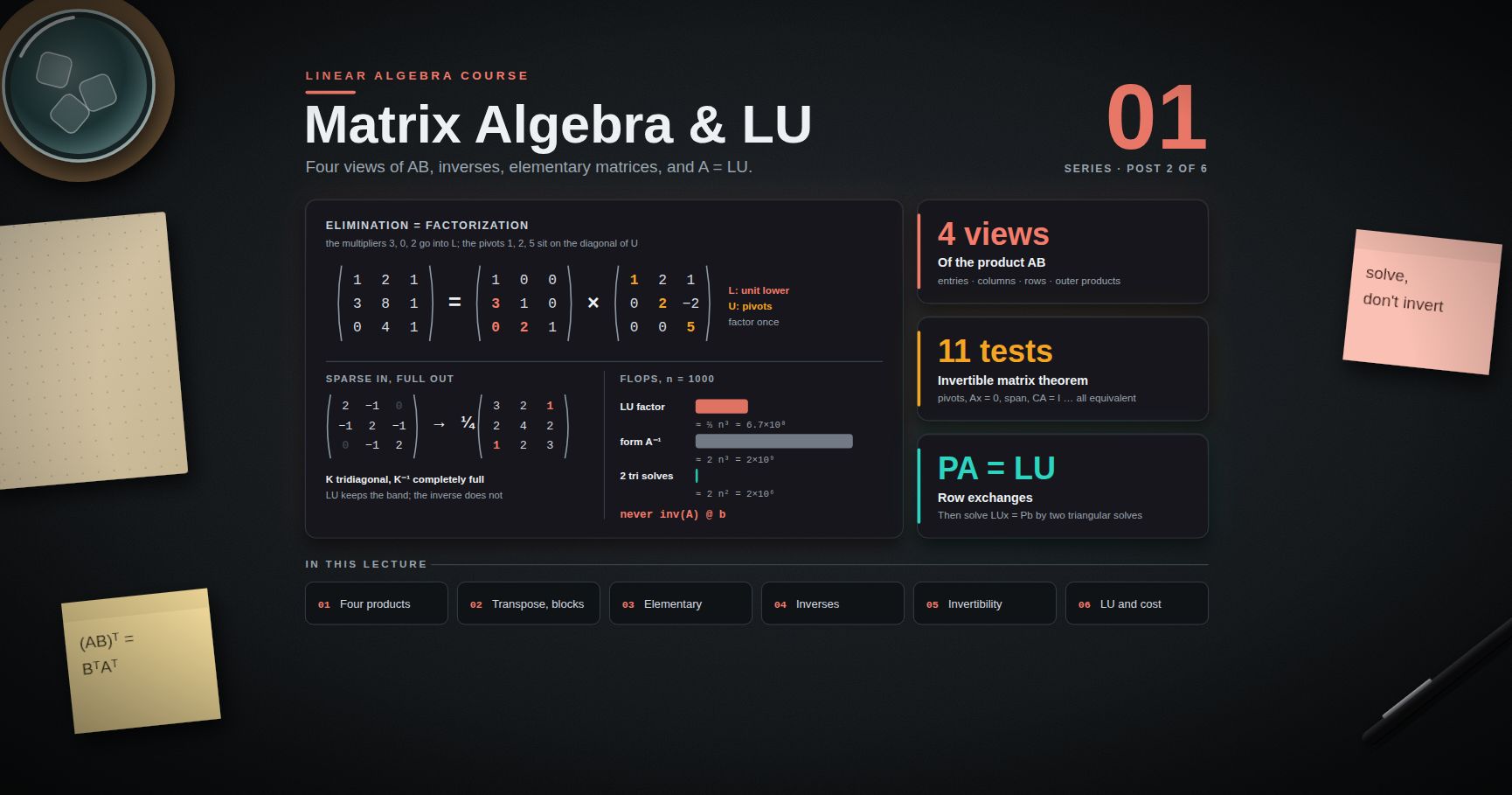
Linear Algebra — 01 · Matrix Algebra, Inverses and LU Factorization
In Linear Algebra 00 a matrix was only a compact way to write a system of equations. This post treats matrices as objects with their own algebra: they can be added, multiplied, transposed and — sometimes — inverted. Matrix multiplication is the operation that makes all of this interesting, so it gets four separate readings, each useful in a different situation. Then row operations become matrices themselves (elementary matrices), which turns Gaussian elimination into an algebraic statement: $A = LU$, a lower triangular matrix times an upper triangular one, or $PA = LU$ when rows must be exchanged. This factorization is how real software solves $A\mathbf{x} = \mathbf{b}$, and it explains a rule every numerical programmer learns early: do not compute $A^{-1}$ to solve a linear system.
> Series map: 00 Vectors & Linear Systems → 01 Matrix Algebra, Inverses & LU (this post) → 02 Vector Spaces, Basis & Dimension → 03 Linear Maps, Change of Basis & Determinants → 04 Eigenvalues & Diagonalization → 05 Inner Products, Spectral Theorem & SVD.
Learning Outcome
- Multiply matrices in four ways — entry by entry, by columns, by rows, and as a sum of outer products — and know when each view is the helpful one.- Explain why $AB \neq BA$ in general, and name other rules from ordinary algebra that fail for matrices.- Use the transpose rules, including $(AB)^T = B^TA^T$, and recognise symmetric, triangular and permutation matrices.- Multiply block (partitioned) matrices and do one step of block elimination.- Write each row operation as an elementary matrix and invert it.- Define the inverse, use the $2 \times 2$ formula, and compute $A^{-1}$ by Gauss–Jordan on $[\,A \mid I\,]$.- State and prove the first version of the invertible matrix theorem.- Factor $A = LU$ and $PA = LU$ by hand, prove that the LU factors are unique, and solve systems with two triangular solves.- Count the cost of elimination (about $\tfrac23 n^3$ flops) and explain why solving with $A^{-1}$ is slower and less reliable.
Chapter 1 — Matrix operations
Terminology
- $m \times n$ matrix — a rectangular array of numbers with $m$ rows and $n$ columns. $a{ij}$ is the entry in row $i$, column $j$.- Square matrix — $m = n$. Its main diagonal is $a{11}, a{22}, \dots, a{nn}$.- Identity matrix $In$ — square, 1 on the main diagonal, 0 elsewhere. $In\mathbf{x} = \mathbf{x}$ for all $\mathbf{x}$.- Zero matrix $0$ — all entries 0.- Equal matrices — same size and the same entry in every position.
Addition and scalar multiplication work entry by entry, exactly as for vectors, and obey the same eight rules. Only matrices of the same size can be added.
The matrix product
If $A$ is $m \times n$ and $B$ is $n \times p$, the product $AB$ is the $m \times p$ matrix with entries
$$(AB){ij} = \sum{k=1}^{n} a{ik} b{kj} = a{i1}b{1j} + a{i2}b{2j} + \dots + a{in}b{nj}.$$
The inner sizes must match: $(m \times n)(n \times p) = m \times p$. The example used throughout this chapter:
$$A = \begin{pmatrix} 1 & 2 \\ 3 & 4 \end{pmatrix}, \qquadB = \begin{pmatrix} 5 & 6 \\ 7 & 8 \end{pmatrix}, \qquadAB = \begin{pmatrix} 19 & 22 \\ 43 & 50 \end{pmatrix}.$$
Four ways to read AB
1. Entry by entry (row times column). $(AB){ij}$ is the dot product of row $i$ of $A$ with column $j$ of $B$. For example $(AB){12} = 1\cdot 6 + 2 \cdot 8 = 22$.
2. By columns. Column $j$ of $AB$ is $A$ times column $j$ of $B$:
$$AB = A\begin{pmatrix} \mathbf{b}1 & \cdots & \mathbf{b}p \end{pmatrix} = \begin{pmatrix} A\mathbf{b}1 & \cdots & A\mathbf{b}p \end{pmatrix}.$$
So every column of $AB$ is a combination of the columns of $A$. Here $A\mathbf{b}1 = 5(1,3) + 7(2,4) = (19, 43)$.
3. By rows. Row $i$ of $AB$ is row $i$ of $A$ times $B$, so every row of $AB$ is a combination of the rows of $B$. Here row 1 is $1\cdot(5,6) + 2\cdot(7,8) = (19, 22)$. This is the view that explains elimination: row operations combine rows.
4. Columns times rows (sum of outer products). Multiply column $k$ of $A$ (an $m \times 1$ matrix) by row $k$ of $B$ (a $1 \times p$ matrix). Each such product is a full $m \times p$ matrix of rank at most one (Linear Algebra 02), and $AB$ is their sum:
$$AB = \sum{k=1}^{n} \mathbf{a}k \mathbf{b}^{}k= \begin{pmatrix} 1 \\ 3 \end{pmatrix}\begin{pmatrix} 5 & 6 \end{pmatrix} + \begin{pmatrix} 2 \\ 4 \end{pmatrix}\begin{pmatrix} 7 & 8 \end{pmatrix}= \begin{pmatrix} 5 & 6 \\ 15 & 18 \end{pmatrix} + \begin{pmatrix} 14 & 16 \\ 28 & 32 \end{pmatrix}= \begin{pmatrix} 19 & 22 \\ 43 & 50 \end{pmatrix}.$$
Here $\mathbf{b}^{}k$ denotes row $k$ of $B$. This view reappears in the SVD (Linear Algebra 05), which writes a matrix as a sum of rank-one pieces ordered by importance.
All four give the same numbers because each one computes $\sumk a{ik}b{kj}$ in position $(i,j)$; they only group the work differently.
> Trick: pick the view that matches the question. "Is $\mathbf{b}$ in the column space?" — columns. "What does a row operation do?" — rows. "What is the rank of $AB$?" — outer products. "Just give me a number" — entries.
Algebraic rules — and what fails
For matrices of compatible sizes:
- $A(BC) = (AB)C$ (associative), $A(B + C) = AB + AC$ and $(A + B)C = AC + BC$ (distributive), $c(AB) = (cA)B = A(cB)$, and $ImA = A = AIn$.
Proof of associativity. For a vector $\mathbf{x}$, $B\mathbf{x} = \sumk xk\mathbf{b}k$, so $A(B\mathbf{x}) = \sumk xk A\mathbf{b}k = (AB)\mathbf{x}$ by the column view. Apply this to each column $\mathbf{c}j$ of $C$: column $j$ of $A(BC)$ is $A(B\mathbf{c}j) = (AB)\mathbf{c}j$, which is column $j$ of $(AB)C$. $\blacksquare$
Three rules from ordinary algebra fail:
1. Not commutative. $BA = \begin{pmatrix} 23 & 34 \\ 31 & 46 \end{pmatrix} \neq AB$. (Often only one of $AB$, $BA$ is even defined.)2. Zero divisors. With $N = \begin{pmatrix} 0 & 1 \\ 0 & 0 \end{pmatrix}$, $N \neq 0$ but $N^2 = 0$.3. No cancellation. $AB = AC$ does not imply $B = C$, even when $A \neq 0$ (take $A = N$, $B = N$, $C = 0$).
> Common pitfall: $(A + B)^2 = A^2 + AB + BA + B^2$, not $A^2 + 2AB + B^2$. The two agree only when $AB = BA$.
Chapter 2 — Transpose and special matrices
Transpose
The transpose $A^T$ of an $m \times n$ matrix is the $n \times m$ matrix with $(A^T){ij} = a{ji}$: rows become columns. Rules:
$$(A^T)^T = A, \qquad (A + B)^T = A^T + B^T, \qquad (cA)^T = cA^T, \qquad (AB)^T = B^TA^T.$$
Proof of the last rule. $((AB)^T){ij} = (AB){ji} = \sumk a{jk}b{ki} = \sumk (B^T){ik}(A^T){kj} = (B^TA^T){ij}$. $\blacksquare$
The order reverses, just like taking off shoes and socks. The dot product is a matrix product: $\mathbf{x}\cdot\mathbf{y} = \mathbf{x}^T\mathbf{y}$ (a $1 \times 1$ matrix).
Special matrices
| Type | Definition | Useful facts ||---|---|---|| Diagonal | $a{ij} = 0$ for $i \neq j$ | products and powers act entry by entry on the diagonal || Upper triangular | $a{ij} = 0$ for $i > j$ | product of two upper triangular is upper triangular || Lower triangular | $a{ij} = 0$ for $i < j$ | same for lower; unit lower triangular has 1s on the diagonal || Symmetric | $A^T = A$ | $A^TA$ and $AA^T$ are always symmetric || Permutation | the rows of $I$ in some order | $P\!A$ reorders the rows of $A$; $P^{-1} = P^T$ |
$A^TA$ is symmetric: $(A^TA)^T = A^T(A^T)^T = A^TA$. For example, with $X = \begin{pmatrix} 1 & 2 \\ 3 & 4 \\ 5 & 6 \end{pmatrix}$, $X^TX = \begin{pmatrix} 35 & 44 \\ 44 & 56 \end{pmatrix}$. This matrix is the heart of least squares (Linear Algebra 05).
Product of lower triangular matrices is lower triangular. If $a{ik} = 0$ for $k > i$ and $b{kj} = 0$ for $j > k$, then in $(AB){ij} = \sumk a{ik}b{kj}$ a term can be nonzero only if $j \le k \le i$. When $i < j$ there is no such $k$, so $(AB){ij} = 0$. If both have unit diagonal, $(AB){ii} = a{ii}b{ii} = 1$. $\blacksquare$
Permutation matrices. Each row and each column of $P$ has exactly one 1. The rows of $P$ are orthonormal, so $PP^T = I$, which means $P^{-1} = P^T$.
Chapter 3 — Block matrices
A matrix can be cut by horizontal and vertical lines into blocks (submatrices). If the column cuts of $A$ match the row cuts of $B$, then $AB$ can be computed block by block, using the same formula as for numbers — but keeping the order of each product:
$$\begin{pmatrix} A{11} & A{12} \\ A{21} & A{22} \end{pmatrix}\begin{pmatrix} B{11} & B{12} \\ B{21} & B{22} \end{pmatrix}=\begin{pmatrix} A{11}B{11} + A{12}B{21} & A{11}B{12} + A{12}B{22} \\ A{21}B{11} + A{22}B{21} & A{21}B{12} + A{22}B{22} \end{pmatrix}.$$
The four views of Chapter 1 are all special cases: the column view cuts $B$ into columns, the row view cuts $A$ into rows, and the outer-product view cuts $A$ into columns and $B$ into rows.
Block elimination and the Schur complement
Let $M = \begin{pmatrix} A & B \\ C & D \end{pmatrix}$ with $A$ square and invertible. Eliminating the block $C$ is one block row operation — "block row 2 minus $CA^{-1}$ times block row 1":
$$\begin{pmatrix} I & 0 \\ -CA^{-1} & I \end{pmatrix}\begin{pmatrix} A & B \\ C & D \end{pmatrix}=\begin{pmatrix} A & B \\ 0 & D - CA^{-1}B \end{pmatrix}.$$
The block $S = D - CA^{-1}B$ is the Schur complement of $A$ in $M$. When every block is $1 \times 1$ this is exactly one step of ordinary elimination: $d - (c/a)b$. Schur complements appear in statistics (conditional covariance), in optimization and in domain-decomposition solvers.
> Watch out: in block formulas every product must keep its order. $CA^{-1}B$ cannot be rewritten as $A^{-1}BC$ or $BCA^{-1}$.
Chapter 4 — Elementary matrices
An elementary matrix is the result of one row operation on the identity. Multiplying $A$ on the left by $E$ performs that row operation on $A$ (by the row view: row $i$ of $EA$ is row $i$ of $E$ times $A$).
Using the $3 \times 3$ system from Linear Algebra 00,
$$A = \begin{pmatrix} 1 & 2 & 1 \\ 3 & 8 & 1 \\ 0 & 4 & 1 \end{pmatrix}, \qquadE{21} = \begin{pmatrix} 1 & 0 & 0 \\ -3 & 1 & 0 \\ 0 & 0 & 1 \end{pmatrix}, \qquadE{32} = \begin{pmatrix} 1 & 0 & 0 \\ 0 & 1 & 0 \\ 0 & -2 & 1 \end{pmatrix}.$$
$E{21}$ subtracts 3 times row 1 from row 2; $E{32}$ subtracts 2 times row 2 from row 3. (No $E{31}$ is needed because $a{31}$ is already 0.) Then
$$E{32}E{21}A = \begin{pmatrix} 1 & 2 & 1 \\ 0 & 2 & -2 \\ 0 & 0 & 5 \end{pmatrix} = U.$$
Every elementary matrix is invertible, and its inverse is elementary of the same type: undo "subtract $\ell$ times row $j$" by "add $\ell$ times row $j$"; undo a swap by the same swap; undo scaling by $c$ by scaling by $1/c$. For example
$$E{21}^{-1} = \begin{pmatrix} 1 & 0 & 0 \\ 3 & 1 & 0 \\ 0 & 0 & 1 \end{pmatrix}.$$
The product in the "wrong" order is messy
$$E{32}E{21} = \begin{pmatrix} 1 & 0 & 0 \\ -3 & 1 & 0 \\ 6 & -2 & 1 \end{pmatrix},\qquadE{21}^{-1}E{32}^{-1} = \begin{pmatrix} 1 & 0 & 0 \\ 3 & 1 & 0 \\ 0 & 2 & 1 \end{pmatrix}.$$
The entry 6 in the first product appears because row 3 is changed using the new row 2, which already contains $-3$ times row 1; indeed $6 = (-2)(-3)$. The inverses, multiplied in the opposite order, do not interact at all: the multipliers $3$ and $2$ simply drop into place. That clean matrix is $L$, and Chapter 7 is built on it. (The messy product $E{32}E{21}$ is $L^{-1}$.)
Chapter 5 — The inverse of a matrix
Definition and uniqueness
A square $n \times n$ matrix $A$ is invertible (or nonsingular) if there is a matrix $C$ with
$$CA = I \quad \text{and} \quad AC = I.$$
Then $C$ is called the inverse and written $A^{-1}$. A square matrix without an inverse is singular.
The inverse is unique. If $CA = I$ and $AD = I$, then $C = CI = C(AD) = (CA)D = ID = D$. $\blacksquare$ (This short argument even shows a left inverse and a right inverse must agree.)
Properties. If $A$ and $B$ are invertible $n \times n$ matrices, then
$$(A^{-1})^{-1} = A, \qquad (AB)^{-1} = B^{-1}A^{-1}, \qquad (A^T)^{-1} = (A^{-1})^T.$$
Proof. $(AB)(B^{-1}A^{-1}) = A(BB^{-1})A^{-1} = AA^{-1} = I$, and similarly in the other order. For the transpose, take the transpose of $AA^{-1} = I$: $(A^{-1})^TA^T = I$, and similarly $A^T(A^{-1})^T = I$. $\blacksquare$
If $A$ is invertible, $A\mathbf{x} = \mathbf{b}$ has exactly one solution for every $\mathbf{b}$, namely $\mathbf{x} = A^{-1}\mathbf{b}$: it is a solution because $A(A^{-1}\mathbf{b}) = \mathbf{b}$, and it is the only one because $A\mathbf{x} = \mathbf{b}$ implies $\mathbf{x} = A^{-1}A\mathbf{x} = A^{-1}\mathbf{b}$.
The 2 × 2 formula
$$\begin{pmatrix} a & b \\ c & d \end{pmatrix}^{-1} = \frac{1}{ad - bc}\begin{pmatrix} d & -b \\ -c & a \end{pmatrix}, \qquad \text{provided } ad - bc \neq 0.$$
Proof. Multiply: $\begin{pmatrix} a & b \\ c & d \end{pmatrix}\begin{pmatrix} d & -b \\ -c & a \end{pmatrix} = \begin{pmatrix} ad - bc & 0 \\ 0 & ad - bc \end{pmatrix}$, and the same holds in the other order. Divide by $ad - bc$. If $ad - bc = 0$, the same product shows $A$ times a matrix gives $0$; Exercise 6 shows $A$ is then singular. $\blacksquare$
The number $ad - bc$ is the determinant of the $2 \times 2$ matrix (Linear Algebra 03 defines it for all sizes). For $A = \begin{pmatrix} 1 & 2 \\ 3 & 4 \end{pmatrix}$: $ad - bc = 4 - 6 = -2$, so
$$A^{-1} = -\frac12 \begin{pmatrix} 4 & -2 \\ -3 & 1 \end{pmatrix} = \begin{pmatrix} -2 & 1 \\ 3/2 & -1/2 \end{pmatrix}.$$
Gauss–Jordan on [ A | I ]
Why it works. Suppose row operations $E1, \dots, Ek$ turn $A$ into $I$: $Ek \cdots E1 A = I$. Then $Ek\cdots E1$ is a left inverse of $A$, and (by the invertible matrix theorem below) it is $A^{-1}$. Applying the same operations to $I$ produces $Ek \cdots E1 I = A^{-1}$. So: row reduce the wide matrix $[\,A \mid I\,]$; if the left half becomes $I$, the right half is $A^{-1}$. If the left half develops a zero row, $A$ is singular.
Worked example. Take the "second difference" matrix
$$K = \begin{pmatrix} 2 & -1 & 0 \\ -1 & 2 & -1 \\ 0 & -1 & 2 \end{pmatrix}.$$
Forward elimination: $R2 \leftarrow R2 + \tfrac12 R1$, then $R3 \leftarrow R3 + \tfrac23 R2$:
$$\left(\begin{array}{ccc|ccc} 2 & -1 & 0 & 1 & 0 & 0 \\ 0 & 3/2 & -1 & 1/2 & 1 & 0 \\ 0 & 0 & 4/3 & 1/3 & 2/3 & 1 \end{array}\right).$$
The pivots are $2, \tfrac32, \tfrac43$. Backward elimination: $R2 \leftarrow R2 + \tfrac34 R3$, then $R1 \leftarrow R1 + \tfrac23 R2$:
$$\left(\begin{array}{ccc|ccc} 2 & 0 & 0 & 3/2 & 1 & 1/2 \\ 0 & 3/2 & 0 & 3/4 & 3/2 & 3/4 \\ 0 & 0 & 4/3 & 1/3 & 2/3 & 1 \end{array}\right).$$
Divide each row by its pivot:
$$K^{-1} = \begin{pmatrix} 3/4 & 1/2 & 1/4 \\ 1/2 & 1 & 1/2 \\ 1/4 & 1/2 & 3/4 \end{pmatrix} = \frac14\begin{pmatrix} 3 & 2 & 1 \\ 2 & 4 & 2 \\ 1 & 2 & 3 \end{pmatrix}.$$
Two observations that matter later. $K$ is symmetric and so is $K^{-1}$ (Exercise 7). And $K$ is tridiagonal — mostly zeros — but $K^{-1}$ is completely full. Keep that in mind for Chapter 8.
Chapter 6 — The invertible matrix theorem
Theorem. For a square $n \times n$ matrix $A$, the following are equivalent (all true or all false):
1. $A$ is invertible.2. $A$ is row equivalent to $In$.3. $A$ has $n$ pivot positions.4. $A\mathbf{x} = \mathbf{0}$ has only the trivial solution.5. The columns of $A$ are linearly independent.6. $A\mathbf{x} = \mathbf{b}$ has at least one solution for every $\mathbf{b} \in \mathbb{R}^n$.7. The columns of $A$ span $\mathbb{R}^n$.8. There is an $n \times n$ matrix $C$ with $CA = I$.9. There is an $n \times n$ matrix $D$ with $AD = I$.10. $A^T$ is invertible.11. $A$ is a product of elementary matrices.
Proof. (1) ⇒ (8) and (1) ⇒ (9): take $C = D = A^{-1}$.
(8) ⇒ (4): if $A\mathbf{x} = \mathbf{0}$ then $\mathbf{x} = CA\mathbf{x} = C\mathbf{0} = \mathbf{0}$.
(4) ⇔ (5): this is the definition of independence (Linear Algebra 00, Chapter 8).
(4) ⇒ (3): only the trivial solution means no free variables, so every one of the $n$ columns is a pivot column.
(3) ⇒ (2): $n$ pivots in an $n \times n$ matrix means one pivot in every row and every column, on the diagonal, so the RREF is $In$.
(2) ⇒ (11): $Ek\cdots E1A = I$ gives $A = E1^{-1}\cdots Ek^{-1}$, a product of elementary matrices.
(11) ⇒ (1): elementary matrices are invertible, and so is any product of invertible matrices.
(9) ⇒ (6): given $\mathbf{b}$, the vector $\mathbf{x} = D\mathbf{b}$ satisfies $A\mathbf{x} = AD\mathbf{b} = \mathbf{b}$.
(6) ⇔ (7): $A\mathbf{x}$ ranges over all combinations of the columns (Linear Algebra 00).
(6) ⇒ (3): if $A$ had fewer than $n$ pivots, its echelon form $U$ would have a zero last row. Choose $\mathbf{c}$ with last entry 1; then $U\mathbf{x} = \mathbf{c}$ is inconsistent, and undoing the row operations on $\mathbf{c}$ gives a $\mathbf{b}$ with $A\mathbf{x} = \mathbf{b}$ inconsistent, contradicting (6).
(1) ⇔ (10): if $A$ is invertible, $(A^{-1})^T$ inverts $A^T$ (Chapter 5); apply this to $A^T$ for the converse.
Every statement is now linked to every other. $\blacksquare$
Corollary (one-sided is enough). If $A$ and $B$ are square and $AB = I$, then $BA = I$ and $B = A^{-1}$. Proof: $AB = I$ is statement (9) for $A$, so $A$ is invertible; multiply $AB = I$ on the left by $A^{-1}$ to get $B = A^{-1}$. $\blacksquare$
> Watch out: the corollary needs square matrices. For $A = \begin{pmatrix} 1 & 0 \end{pmatrix}$ and $B = \begin{pmatrix} 1 \\ 0 \end{pmatrix}$, $AB = (1) = I1$ but $BA = \begin{pmatrix} 1 & 0 \\ 0 & 0 \end{pmatrix} \neq I2$.
Linear Algebra 02, 03 and 04 add more lines to this list: rank $n$, null space $\{\mathbf{0}\}$, $\det A \neq 0$, and $0$ is not an eigenvalue.
Chapter 7 — LU factorization
From elimination to A = LU
Suppose elimination on $A$ needs no row exchanges. Then only replacement operations "row $i$ minus $\ell{ij}$ times row $j$" (with $i > j$) are used, and
$$(E{32}E{31}E{21})\,A = U \qquad\Longrightarrow\qquad A = (E{21}^{-1}E{31}^{-1}E{32}^{-1})\,U = LU$$
(written for $n = 3$; larger $n$ is the same). $U$ is upper triangular with the pivots on its diagonal. $L$ is unit lower triangular, and as Chapter 4 showed, its entries below the diagonal are exactly the multipliers: $L{ij} = \ell{ij}$.
For the running example, the multipliers were $\ell{21} = 3$, $\ell{31} = 0$, $\ell{32} = 2$, so
$$\begin{pmatrix} 1 & 2 & 1 \\ 3 & 8 & 1 \\ 0 & 4 & 1 \end{pmatrix}=\begin{pmatrix} 1 & 0 & 0 \\ 3 & 1 & 0 \\ 0 & 2 & 1 \end{pmatrix}\begin{pmatrix} 1 & 2 & 1 \\ 0 & 2 & -2 \\ 0 & 0 & 5 \end{pmatrix}.$$
Multiply it out to check: row 2 of $LU$ is $3(1,2,1) + (0,2,-2) = (3, 8, 1)$, and row 3 is $2(0,2,-2) + (0,0,5) = (0, 4, 1)$.
Solving with L and U
$A\mathbf{x} = \mathbf{b}$ becomes $L(U\mathbf{x}) = \mathbf{b}$. Put $\mathbf{c} = U\mathbf{x}$ and solve two triangular systems:
1. Forward substitution $L\mathbf{c} = \mathbf{b}$ (top to bottom).2. Back substitution $U\mathbf{x} = \mathbf{c}$ (bottom to top).
With $\mathbf{b} = (2, 12, 2)$: $c1 = 2$; $3c1 + c2 = 12$ gives $c2 = 6$; $2c2 + c3 = 2$ gives $c3 = -10$. So $\mathbf{c} = (2, 6, -10)$ — exactly the right-hand side that elimination produced in Linear Algebra 00. Then $U\mathbf{x} = \mathbf{c}$ gives $z = -2$, $y = 1$, $x = 2$, as before.
The point: the factorization is done once; each new right-hand side then costs only two cheap triangular solves.
LDU and the symmetric case
Divide each row of $U$ by its pivot to get $A = LDU'$ with $D$ the diagonal matrix of pivots and $U'$ unit upper triangular. For the example, $D = \operatorname{diag}(1, 2, 5)$ and
$$U' = \begin{pmatrix} 1 & 2 & 1 \\ 0 & 1 & -1 \\ 0 & 0 & 1 \end{pmatrix}.$$
When $A$ is symmetric and has an LU factorization, $U' = L^T$, so $A = LDL^T$. For a symmetric matrix with all pivots positive this becomes the Cholesky factorization $A = (LD^{1/2})(LD^{1/2})^T$, which costs about half as much as LU.
Uniqueness
Theorem. If $A$ is invertible and $A = L1U1 = L2U2$ with $L1, L2$ unit lower triangular and $U1, U2$ upper triangular, then $L1 = L2$ and $U1 = U2$.
Proof. Since $A$ is invertible, so are the $Ui$ (and the unit-diagonal $Li$ always are). From $L1U1 = L2U2$,
$$L2^{-1}L1 = U2U1^{-1}.$$
The left side is unit lower triangular (inverses and products of unit lower triangular matrices are unit lower triangular — Chapter 2 and Exercise 5), and the right side is upper triangular. A matrix that is both is diagonal, and its diagonal is all 1s from the left side. So both sides equal $I$, which gives $L1 = L2$ and $U1 = U2$. $\blacksquare$
Row exchanges: PA = LU
Elimination breaks down when a zero appears in a pivot position. Example:
$$A = \begin{pmatrix} 0 & 1 & 1 \\ 1 & 2 & 1 \\ 2 & 7 & 9 \end{pmatrix}.$$
The (1,1) entry is 0, so swap rows 1 and 2 first. If all the exchanges are done at the start, they form one permutation matrix $P$, and $PA$ factors without further trouble:
$$P = \begin{pmatrix} 0 & 1 & 0 \\ 1 & 0 & 0 \\ 0 & 0 & 1 \end{pmatrix}, \qquadPA = \begin{pmatrix} 1 & 2 & 1 \\ 0 & 1 & 1 \\ 2 & 7 & 9 \end{pmatrix}= \begin{pmatrix} 1 & 0 & 0 \\ 0 & 1 & 0 \\ 2 & 3 & 1 \end{pmatrix}\begin{pmatrix} 1 & 2 & 1 \\ 0 & 1 & 1 \\ 0 & 0 & 4 \end{pmatrix}.$$
The multipliers were $\ell{21} = 0$, $\ell{31} = 2$ (row 3 becomes $(0, 3, 7)$), then $\ell{32} = 3$ (row 3 becomes $(0, 0, 4)$).
Theorem. For every invertible $A$ there is a permutation matrix $P$ such that $PA = LU$ with $L$ unit lower triangular and $U$ upper triangular with nonzero pivots. An invertible $A$ has an LU factorization with no exchanges ($P = I$) exactly when every leading principal submatrix (the top-left $k \times k$ block, $k = 1, \dots, n$) is invertible.
To solve $A\mathbf{x} = \mathbf{b}$ from $PA = LU$: $LU\mathbf{x} = P\mathbf{b}$, so permute $\mathbf{b}$, then do the two triangular solves.
> Common pitfall: after factoring $PA = LU$, forgetting to apply $P$ to $\mathbf{b}$. The factorization is of $PA$, not of $A$.
Chapter 8 — Cost, and why not to compute the inverse
Counting flops
A flop is one floating-point add, subtract, multiply or divide. At elimination step $k$ of an $n \times n$ matrix, each of the $n - k$ rows below the pivot needs one division (its multiplier) and a multiply and a subtract for each of the remaining $n - k$ entries. So step $k$ costs $(n - k)\bigl(2(n - k) + 1\bigr)$ flops, and in total
$$\sum{k=1}^{n} \bigl( 2(n-k)^2 + (n-k) \bigr) = \frac{2}{3}n^3 - \frac12 n^2 - \frac16 n \approx \frac23 n^3.$$
Each triangular solve costs about $n^2$ flops. So for $n = 1000$: roughly $6.7 \times 10^8$ flops to factor, then only about $2 \times 10^6$ per right-hand side.
Why solving with the inverse is the wrong way
1. Speed. Forming $A^{-1}$ costs about $2n^3$ flops — roughly three times the LU factorization — and then $A^{-1}\mathbf{b}$ still costs $2n^2$, the same as the two triangular solves it was supposed to replace. There is nothing to gain even with many right-hand sides, because LU is reusable too.2. Accuracy. Gaussian elimination with partial pivoting is backward stable in practice: the computed $\mathbf{x}$ exactly solves a system with a very slightly perturbed $A$. Multiplying by a computed inverse does not have this guarantee in general, and its residual $\lVert \mathbf{b} - A\mathbf{x} \rVert$ is typically larger (Higham, Chapters 9 and 14).3. Structure. A banded or sparse matrix has banded or sparse LU factors (without pivoting, a tridiagonal $K$ has bidiagonal $L$ and $U$), but its inverse is usually full — as $K^{-1}$ in Chapter 5 showed. For large sparse problems the inverse may not even fit in memory.
In code this means (which calls LAPACK's LU-based ), or once and for each right-hand side — never .
> Trick: read $A^{-1}\mathbf{b}$ in a formula as "the solution of $A\mathbf{x} = \mathbf{b}$", not as an instruction to invert. The same holds for expressions like $A^{-1}B$ (solve with many right-hand sides) and $\mathbf{c}^TA^{-1}\mathbf{b}$ (one solve, then one dot product).
Practice Exercises
Exercise 1 — Order matters
Let $A = \begin{pmatrix} 1 & 0 \\ 2 & 1 \end{pmatrix}$ and $B = \begin{pmatrix} 3 & 1 \\ 0 & 2 \end{pmatrix}$. Compute $AB$ and $BA$. Describe $AB$ with the row view.
<details><summary>Solution</summary>
$AB = \begin{pmatrix} 3 & 1 \\ 6 & 4 \end{pmatrix}$ and $BA = \begin{pmatrix} 5 & 1 \\ 4 & 2 \end{pmatrix}$, which differ. Row view: $A$ is an elementary matrix ("add 2 times row 1 to row 2"), so $AB$ is $B$ with row 2 replaced by $(0,2) + 2(3,1) = (6, 4)$.
</details>
Exercise 2 — Transpose of a triple product
Prove $(ABC)^T = C^TB^TA^T$, and deduce that $B^TAB$ is symmetric whenever $A$ is symmetric.
<details><summary>Solution</summary>
$(ABC)^T = ((AB)C)^T = C^T(AB)^T = C^TB^TA^T$. If $A^T = A$, then $(B^TAB)^T = B^TA^T(B^T)^T = B^TAB$.
</details>
Exercise 3 — Inverses
Find the inverse of $\begin{pmatrix} 2 & 5 \\ 1 & 3 \end{pmatrix}$ with the $2 \times 2$ formula, and of $\begin{pmatrix} 1 & 2 & 3 \\ 0 & 1 & 4 \\ 5 & 6 & 0 \end{pmatrix}$ by Gauss–Jordan.
<details><summary>Solution</summary>
$ad - bc = 6 - 5 = 1$, so the first inverse is $\begin{pmatrix} 3 & -5 \\ -1 & 2 \end{pmatrix}$.
For the $3 \times 3$ matrix, row reducing $[\,A \mid I\,]$ gives
$$A^{-1} = \begin{pmatrix} -24 & 18 & 5 \\ 20 & -15 & -4 \\ -5 & 4 & 1 \end{pmatrix}.$$
Check one entry of $AA^{-1}$: row 3 of $A$ times column 1 of $A^{-1}$ is $5(-24) + 6(20) + 0 = 0$, as it should be.
</details>
Exercise 4 — LU by hand
Factor $A = \begin{pmatrix} 2 & 1 & 1 \\ 4 & -6 & 0 \\ -2 & 7 & 2 \end{pmatrix}$ as $LU$.
<details><summary>Solution</summary>
$\ell{21} = 4/2 = 2$ and $\ell{31} = -2/2 = -1$ give rows $(0, -8, -2)$ and $(0, 8, 3)$. Then $\ell{32} = 8/(-8) = -1$ gives row 3 $= (0, 0, 1)$. So
$$L = \begin{pmatrix} 1 & 0 & 0 \\ 2 & 1 & 0 \\ -1 & -1 & 1 \end{pmatrix}, \qquadU = \begin{pmatrix} 2 & 1 & 1 \\ 0 & -8 & -2 \\ 0 & 0 & 1 \end{pmatrix}.$$
Pivots $2, -8, 1$.
</details>
Exercise 5 — Inverse of a unit lower triangular matrix
Show that the inverse of a unit lower triangular matrix is unit lower triangular (this completes the uniqueness proof in Chapter 7).
<details><summary>Solution</summary>
A unit lower triangular $L$ reduces to $I$ using only operations "row $i$ minus a multiple of row $j$" with $i > j$ (no swaps, no scaling, since the pivots are already 1). Each such elementary matrix is unit lower triangular, so $L^{-1}$, the product of these elementary matrices, is unit lower triangular by the Chapter 2 result.
</details>
Exercise 6 — A zero pivot that cannot be fixed
Show that if $ad - bc = 0$ then $A = \begin{pmatrix} a & b \\ c & d \end{pmatrix}$ is singular. Also show that $\begin{pmatrix} 0 & 1 \\ 1 & 1 \end{pmatrix}$ is invertible but has no LU factorization without a row exchange.
<details><summary>Solution</summary>
If $A = 0$ it is singular. Otherwise $M = \begin{pmatrix} d & -b \\ -c & a \end{pmatrix} \neq 0$ and $AM = 0$. If $A$ were invertible, $M = A^{-1}AM = 0$, a contradiction.
For the second matrix, $ad - bc = -1 \neq 0$, so it is invertible. If $\begin{pmatrix} 0 & 1 \\ 1 & 1 \end{pmatrix} = \begin{pmatrix} 1 & 0 \\ \ell & 1 \end{pmatrix}\begin{pmatrix} u{11} & u{12} \\ 0 & u{22} \end{pmatrix}$, the (1,1) entry forces $u{11} = 0$, but then the (2,1) entry is $\ell u{11} = 0 \neq 1$. Its first leading principal submatrix $(0)$ is singular, as the theorem predicts. With the swap, $PA = \begin{pmatrix} 1 & 1 \\ 0 & 1 \end{pmatrix} = I \cdot U$.
</details>
Exercise 7 — Symmetric inverse
Prove: if $A$ is symmetric and invertible, then $A^{-1}$ is symmetric.
<details><summary>Solution</summary>
$(A^{-1})^T = (A^T)^{-1} = A^{-1}$, using the transpose rule for inverses from Chapter 5 and $A^T = A$.
</details>
Cheat-sheet
| Topic | Key fact ||---|---|| Product size | $(m \times n)(n \times p) = m \times p$ || Four views of $AB$ | entries, columns $A\mathbf{b}j$, rows, sum of outer products || Fails for matrices | $AB = BA$, cancellation, "no zero divisors" || Transpose | $(AB)^T = B^TA^T$; $A^TA$ is symmetric || Block product | same formula as scalars, order kept || Schur complement | $D - CA^{-1}B$ || Elementary matrix | row operation on $I$; multiply on the left || $2 \times 2$ inverse | swap $a, d$; negate $b, c$; divide by $ad - bc \neq 0$ || Inverse rules | $(AB)^{-1} = B^{-1}A^{-1}$, $(A^T)^{-1} = (A^{-1})^T$ || Compute $A^{-1}$ | Gauss–Jordan on $[\,A \mid I\,]$ || Square, $AB = I$ | then $BA = I$ || $A = LU$ | $L$ unit lower with multipliers; $U$ upper with pivots || Row exchanges | $PA = LU$; solve $LU\mathbf{x} = P\mathbf{b}$ || LU cost | $\approx \tfrac23 n^3$ flops; each triangular solve $\approx n^2$ || Solve, do not invert | or + |
What's next
Linear Algebra 02 steps back from matrices to the structures they act on. It defines a vector space by axioms (so polynomials, functions and matrices count), then subspaces, span, independence, basis and dimension — with a full proof that dimension is well defined (the Steinitz exchange lemma). It then studies the four fundamental subspaces of a matrix, proves that row rank equals column rank, and proves rank–nullity in matrix form.
References
- Gilbert Strang, Introduction to Linear Algebra, 6th edition, Wellesley-Cambridge Press, 2023 — Chapter 2 (elimination matrices, inverses, $A = LU$, transposes and permutations).- David C. Lay, Steven R. Lay and Judi J. McDonald, Linear Algebra and Its Applications, 6th edition, Pearson, 2021 — Chapter 2 (matrix operations, the invertible matrix theorem, partitioned matrices, LU).- Lloyd N. Trefethen and David Bau III, Numerical Linear Algebra, SIAM, 1997 — Lectures 20–21 (Gaussian elimination, operation count, pivoting).- Gene H. Golub and Charles F. Van Loan, Matrix Computations, 4th edition, Johns Hopkins University Press, 2013 — Chapter 3 (LU and its variants).- Nicholas J. Higham, Accuracy and Stability of Numerical Algorithms, 2nd edition, SIAM, 2002 — Chapter 9 (LU factorization and linear equations) and Chapter 14 (matrix inversion).- MIT OpenCourseWare, 18.06 Linear Algebra, Spring 2010 (Gilbert Strang) — Lectures 3–5: multiplication and inverses, $A = LU$, transposes and permutations.
> Note: this post is in progress. Planned additions: a proof of the leading-principal-submatrix condition for LU without exchanges, a worked partial-pivoting example in three-digit arithmetic, and a short numerical demo comparing with on an ill-conditioned matrix.
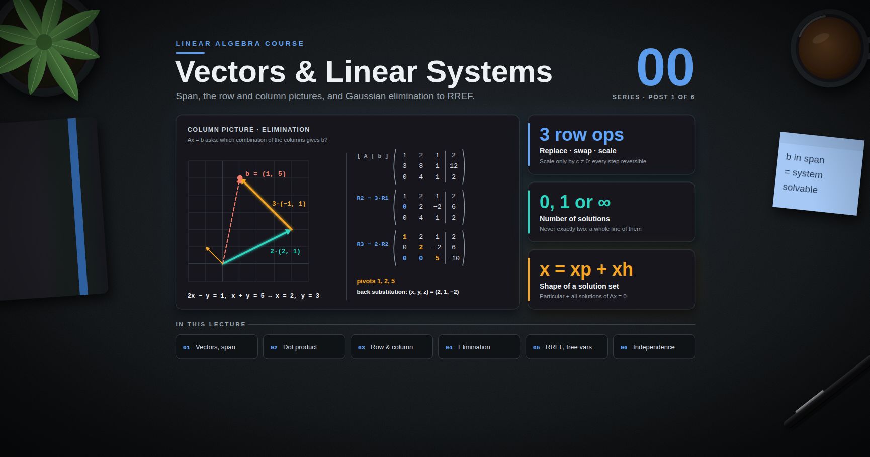
Linear Algebra — 00 · Vectors and Systems of Linear Equations
Linear algebra is the study of vectors, of the linear equations that tie them together, and of the maps that preserve their structure. It is the working language of numerical computing, statistics, machine learning, graphics, quantum mechanics and control, and it is the first course where most students meet mathematics built from definitions and proofs rather than from formulas. This six-post series is written for a reader who knows high-school algebra and wants the full senior-undergraduate picture: computation first, then the abstract theory, with proofs of the key theorems. Post 00 starts at the very beginning — vectors in $\mathbb{R}^n$, linear combinations, span, the dot product, systems of linear equations and Gaussian elimination — and ends with the structure of a solution set and a first look at linear independence. Posts 01–05 cover matrix algebra and LU, vector spaces and dimension, linear maps and determinants, eigenvalues, and inner products through the spectral theorem and the SVD. The standard textbooks behind the series are Strang (computation and the four subspaces), Lay (clear worked examples), Axler (the abstract, determinant-free view) and Hoffman–Kunze (the classical rigorous treatment).
> Series map: 00 Vectors & Linear Systems (this post) → 01 Matrix Algebra, Inverses & LU → 02 Vector Spaces, Basis & Dimension → 03 Linear Maps, Change of Basis & Determinants → 04 Eigenvalues & Diagonalization → 05 Inner Products, Spectral Theorem & SVD.
Learning Outcome
- Add and scale vectors in $\mathbb{R}^n$, and describe a linear combination both algebraically and geometrically.- Describe the span of one, two or three vectors in $\mathbb{R}^3$ as a point, a line, a plane or all of space.- Compute dot products, lengths and angles, and recognise orthogonal vectors.- Read a system $A\mathbf{x} = \mathbf{b}$ in two ways: the row picture (intersecting lines or planes) and the column picture (a combination of columns).- Apply the three elementary row operations and explain why they never change the solution set.- Run Gaussian elimination and Gauss–Jordan elimination by hand, and bring a matrix to row echelon form and to reduced row echelon form.- Identify pivots and free variables, decide consistency, and write every solution in parametric vector form.- Prove that a solution set is "one particular solution plus all homogeneous solutions".- Test a small set of vectors for linear independence.
Notation used in the whole series
| Symbol | Meaning ||---|---|| $\mathbb{R}$, $\mathbb{R}^n$ | real numbers; column vectors with $n$ real entries || $\mathbf{x}, \mathbf{v}, \mathbf{b}$ | vectors (bold lower case), always columns unless stated || $xi$ | the $i$-th entry of $\mathbf{x}$ || $A, B, U$ | matrices (capital letters); $a{ij}$ is the entry in row $i$, column $j$ || $m \times n$ | $m$ rows, $n$ columns || $\mathbf{a}j$ | column $j$ of $A$ || $A^T$ | transpose (rows become columns) || $\mathbf{0}$ | the zero vector || $\mathbf{e}i$ | standard basis vector: 1 in position $i$, 0 elsewhere |
Chapter 1 — Vectors in n-space
Terminology
- Scalar — a single real number. Later in the series scalars may come from any field (see Linear Algebra 02), but for now they are real.- Vector in $\mathbb{R}^n$ — an ordered list of $n$ real numbers, written as a column. The numbers are its entries or components.- Zero vector $\mathbf{0}$ — the vector whose entries are all 0.- Vector addition — add entry by entry. Only defined for two vectors of the same length.- Scalar multiplication — multiply every entry by the same scalar.
$$\mathbf{v} = \begin{pmatrix} v1 \\ v2 \\ \vdots \\ vn \end{pmatrix}, \qquad\mathbf{v} + \mathbf{w} = \begin{pmatrix} v1 + w1 \\ \vdots \\ vn + wn \end{pmatrix}, \qquadc\,\mathbf{v} = \begin{pmatrix} c v1 \\ \vdots \\ c vn \end{pmatrix}.$$
Algebraic rules
For all $\mathbf{u}, \mathbf{v}, \mathbf{w} \in \mathbb{R}^n$ and all scalars $c, d$:
1. $\mathbf{u} + \mathbf{v} = \mathbf{v} + \mathbf{u}$ and $(\mathbf{u} + \mathbf{v}) + \mathbf{w} = \mathbf{u} + (\mathbf{v} + \mathbf{w})$.2. $\mathbf{v} + \mathbf{0} = \mathbf{v}$ and $\mathbf{v} + (-\mathbf{v}) = \mathbf{0}$.3. $c(\mathbf{u} + \mathbf{v}) = c\mathbf{u} + c\mathbf{v}$ and $(c + d)\mathbf{v} = c\mathbf{v} + d\mathbf{v}$.4. $c(d\mathbf{v}) = (cd)\mathbf{v}$ and $1\mathbf{v} = \mathbf{v}$.
Each rule follows from the matching rule for real numbers, applied one entry at a time. These eight rules are exactly the axioms of a vector space; Linear Algebra 02 turns them into a definition, and then polynomials, functions and matrices become "vectors" too.
The geometric picture
In $\mathbb{R}^2$ and $\mathbb{R}^3$ a vector is an arrow from the origin to the point with those coordinates.
- Addition is the parallelogram rule: place the tail of $\mathbf{w}$ at the head of $\mathbf{v}$; the sum ends where $\mathbf{w}$ ends.- Scaling stretches the arrow by $\lvert c\rvert$ and reverses it when $c < 0$.- $\mathbf{v} - \mathbf{w}$ is the arrow from the head of $\mathbf{w}$ to the head of $\mathbf{v}$.
For $n > 3$ there is no picture, but every algebraic fact still holds. The habit to build is: reason with the algebra, check the intuition in $\mathbb{R}^2$ or $\mathbb{R}^3$.
> Watch out: a point and a vector are written the same way in $\mathbb{R}^n$, but they play different roles. A point is a location; a vector is a displacement. The distinction matters in Chapter 7, where a solution set can be a plane that does not pass through the origin.
Chapter 2 — Linear combinations and span
Terminology
- Linear combination of $\mathbf{v}1, \dots, \mathbf{v}k$ — any vector $c1\mathbf{v}1 + c2\mathbf{v}2 + \dots + ck\mathbf{v}k$ with scalars $c1, \dots, ck$ (the weights or coefficients).- Span — the set of all linear combinations:
$$\operatorname{span}\{\mathbf{v}1, \dots, \mathbf{v}k\} = \{\, c1\mathbf{v}1 + \dots + ck\mathbf{v}k : c1, \dots, ck \in \mathbb{R} \,\}.$$
The span always contains $\mathbf{0}$ (take every weight 0) and each $\mathbf{v}i$ itself (weight 1 on it, 0 elsewhere).
Geometric picture of a span in R³
| Vectors | Span ||---|---|| only $\mathbf{0}$ | the single point $\{\mathbf{0}\}$ || one nonzero $\mathbf{v}$ | the line through the origin in direction $\mathbf{v}$ || two vectors, neither a multiple of the other | the plane through the origin containing both || two vectors, one a multiple of the other | still only a line || three vectors not in one plane | all of $\mathbb{R}^3$ || three vectors in one plane | only that plane (or a line) |
The pattern "adding a vector enlarges the span only if the new vector is not already inside it" is the seed of linear independence (Chapter 8) and of dimension (Linear Algebra 02).
Worked example — is b in the span?
Is $\mathbf{b} = (1, 5)$ a combination of $\mathbf{a}1 = (2, 1)$ and $\mathbf{a}2 = (-1, 1)$? We need $x, y$ with
$$x \begin{pmatrix} 2 \\ 1 \end{pmatrix} + y \begin{pmatrix} -1 \\ 1 \end{pmatrix} = \begin{pmatrix} 1 \\ 5 \end{pmatrix}\quad\Longleftrightarrow\quad\begin{aligned} 2x - y &= 1 \\ x + y &= 5. \end{aligned}$$
Adding the two equations gives $3x = 6$, so $x = 2$ and $y = 3$. Check: $2(2,1) + 3(-1,1) = (4-3,\ 2+3) = (1, 5)$. So $\mathbf{b}$ is in the span. In fact, since $\mathbf{a}1$ and $\mathbf{a}2$ are not parallel, their span is the whole plane $\mathbb{R}^2$.
The key lesson: "is $\mathbf{b}$ in the span of these vectors?" is the same question as "does this linear system have a solution?" Everything in this post comes back to that sentence.
Chapter 3 — Dot product and length
This chapter is brief; inner products get their full treatment in Linear Algebra 05.
Definitions
- Dot product: $\mathbf{u} \cdot \mathbf{v} = u1 v1 + u2 v2 + \dots + un vn$. It takes two vectors and returns a scalar.- Length (norm): $\lVert \mathbf{v} \rVert = \sqrt{\mathbf{v} \cdot \mathbf{v}} = \sqrt{v1^2 + \dots + vn^2}$.- Unit vector: a vector of length 1. For $\mathbf{v} \neq \mathbf{0}$, the vector $\mathbf{v} / \lVert \mathbf{v} \rVert$ is the unit vector in the same direction.- Orthogonal: $\mathbf{u}$ and $\mathbf{v}$ are orthogonal (perpendicular) when $\mathbf{u} \cdot \mathbf{v} = 0$.
Properties
The dot product is symmetric ($\mathbf{u}\cdot\mathbf{v} = \mathbf{v}\cdot\mathbf{u}$), linear in each argument, and positive definite: $\mathbf{v}\cdot\mathbf{v} \ge 0$, with equality only for $\mathbf{v} = \mathbf{0}$. Two inequalities hold for all $\mathbf{u}, \mathbf{v} \in \mathbb{R}^n$ (proofs in Linear Algebra 05):
$$\lvert \mathbf{u} \cdot \mathbf{v} \rvert \le \lVert \mathbf{u} \rVert \, \lVert \mathbf{v} \rVert \quad \text{(Cauchy–Schwarz)}, \qquad\lVert \mathbf{u} + \mathbf{v} \rVert \le \lVert \mathbf{u} \rVert + \lVert \mathbf{v} \rVert \quad \text{(triangle inequality)}.$$
Cauchy–Schwarz is what makes the angle formula legitimate: for nonzero vectors the ratio below lies in $[-1, 1]$, so it is the cosine of exactly one angle $\theta \in [0, \pi]$.
$$\cos\theta = \frac{\mathbf{u}\cdot\mathbf{v}}{\lVert \mathbf{u}\rVert\,\lVert \mathbf{v}\rVert}.$$
Worked example
Let $\mathbf{u} = (1, 2, 2)$ and $\mathbf{v} = (2, -2, 1)$. Then $\lVert \mathbf{u} \rVert = \sqrt{1 + 4 + 4} = 3$, so $\mathbf{u}/3 = (1/3, 2/3, 2/3)$ is a unit vector. And $\mathbf{u}\cdot\mathbf{v} = 2 - 4 + 2 = 0$, so $\mathbf{u}$ and $\mathbf{v}$ are orthogonal.
> Trick: the dot product gives a second reading of one equation. The equation $a1x1 + \dots + anxn = b$ says $\mathbf{a}\cdot\mathbf{x} = b$. When $b = 0$, the solutions are exactly the vectors orthogonal to $\mathbf{a}$ — a line in $\mathbb{R}^2$, a plane in $\mathbb{R}^3$, a "hyperplane" in general.
Chapter 4 — Systems of linear equations
Terminology
- Linear equation in $x1, \dots, xn$ — an equation $a1x1 + \dots + anxn = b$ with constant coefficients $ai$ and constant $b$. No products $xixj$, no powers, no $\sin x$.- System of linear equations — a finite list of linear equations in the same unknowns.- Solution — a vector $\mathbf{x}$ that satisfies every equation at once. The solution set is the set of all solutions.- Consistent — has at least one solution. Inconsistent — has none.- Equivalent systems — systems with the same solution set.- Coefficient matrix $A$ — the $m \times n$ array of the $a{ij}$. Augmented matrix $[\,A \mid \mathbf{b}\,]$ — $A$ with $\mathbf{b}$ attached as an extra column.
Matrix times vector
Write the columns of $A$ as $\mathbf{a}1, \dots, \mathbf{a}n$. The product $A\mathbf{x}$ is defined as a combination of the columns, with the entries of $\mathbf{x}$ as weights:
$$A\mathbf{x} = \begin{pmatrix} \mathbf{a}1 & \mathbf{a}2 & \cdots & \mathbf{a}n \end{pmatrix}\begin{pmatrix} x1 \\ \vdots \\ xn \end{pmatrix} = x1\mathbf{a}1 + x2\mathbf{a}2 + \dots + xn\mathbf{a}n.$$
Entry $i$ of that combination is $a{i1}x1 + \dots + a{in}xn$, which is the dot product of row $i$ of $A$ with $\mathbf{x}$. So there are two ways to compute $A\mathbf{x}$ — by columns and by rows — and they always agree. A system of $m$ equations in $n$ unknowns is therefore one vector equation $A\mathbf{x} = \mathbf{b}$, with $A$ of size $m \times n$, $\mathbf{x} \in \mathbb{R}^n$ and $\mathbf{b} \in \mathbb{R}^m$.
Two rules follow straight from the definition and are used constantly: $A(\mathbf{u} + \mathbf{v}) = A\mathbf{u} + A\mathbf{v}$ and $A(c\mathbf{u}) = c\,A\mathbf{u}$.
Row picture and column picture
Take the system from Chapter 2:
$$\begin{aligned} 2x - y &= 1 \\ x + y &= 5 \end{aligned}\qquad\Longleftrightarrow\qquad\begin{pmatrix} 2 & -1 \\ 1 & 1 \end{pmatrix} \begin{pmatrix} x \\ y \end{pmatrix} = \begin{pmatrix} 1 \\ 5 \end{pmatrix}.$$
- Row picture. Each equation is a line in the $xy$-plane: $y = 2x - 1$ and $y = 5 - x$. A solution is a point on both lines. They cross at $(2, 3)$.- Column picture. The same system asks for weights on the columns $(2, 1)$ and $(-1, 1)$ that produce $(1, 5)$. The answer is $2$ of the first column plus $3$ of the second.
The same numbers $x = 2$, $y = 3$ appear in both pictures, but they mean different things: a point where lines cross, or weights in a combination.
In $\mathbb{R}^3$ the row picture has three planes, and a solution is a point common to all three. The column picture has three column vectors in $\mathbb{R}^3$, and the question is whether $\mathbf{b}$ is a combination of them. The column picture scales to any size and becomes the main point of view from Linear Algebra 02 onwards (column space).
How many solutions can there be?
Theorem (zero, one or infinitely many). A linear system has either no solution, exactly one solution, or infinitely many solutions.
Proof. Suppose $\mathbf{x}$ and $\mathbf{y}$ are two different solutions, so $A\mathbf{x} = A\mathbf{y} = \mathbf{b}$. For every real $t$, put $\mathbf{z}t = \mathbf{x} + t(\mathbf{y} - \mathbf{x})$. Then
$$A\mathbf{z}t = A\mathbf{x} + t(A\mathbf{y} - A\mathbf{x}) = \mathbf{b} + t(\mathbf{b} - \mathbf{b}) = \mathbf{b}.$$
Since $\mathbf{y} - \mathbf{x} \neq \mathbf{0}$, different values of $t$ give different vectors $\mathbf{z}t$, so there are infinitely many solutions. $\blacksquare$
Geometrically: the whole line through two solutions consists of solutions. Two lines in the plane cannot meet in exactly two points.
Chapter 5 — Elimination
Elementary row operations
Three operations on the rows of an augmented matrix:
1. Replacement — add a multiple of one row to another row: $Ri \leftarrow Ri + cRj$ (with $i \neq j$).2. Interchange — swap two rows: $Ri \leftrightarrow Rj$.3. Scaling — multiply a row by a nonzero constant: $Ri \leftarrow cRi$, $c \neq 0$.
Two matrices are row equivalent if one can be turned into the other by a finite sequence of these operations.
Theorem. If two augmented matrices are row equivalent, the corresponding systems have the same solution set.
Proof. It is enough to check one operation at a time. Any $\mathbf{x}$ that satisfies the old equations also satisfies the new ones: a swap or a scaling changes nothing essential, and if $\mathbf{x}$ satisfies equations $i$ and $j$ it satisfies their sum "$i + c\cdot j$". Conversely, each operation can be undone by an operation of the same type — replacement by $Ri \leftarrow Ri - cRj$, interchange by the same swap, scaling by $1/c$ (this is why $c \neq 0$ is required). So any solution of the new system also solves the old one. $\blacksquare$
> Common pitfall: multiplying a row by $0$ is not allowed. It destroys an equation and can create new "solutions". Scaling needs $c \neq 0$ precisely so the step is reversible.
Gaussian elimination on a 3 × 3 system
Solve
$$\begin{aligned}x + 2y + z &= 2 \\3x + 8y + z &= 12 \\4y + z &= 2\end{aligned}\qquad[\,A \mid \mathbf{b}\,] = \left(\begin{array}{ccc|c} 1 & 2 & 1 & 2 \\ 3 & 8 & 1 & 12 \\ 0 & 4 & 1 & 2 \end{array}\right).$$
Step 1 — clear column 1 below the first pivot. The first pivot is the 1 in position (1,1). Row 2 needs multiplier $\ell{21} = 3/1 = 3$; row 3 already has a 0, so $\ell{31} = 0$.
$$R2 \leftarrow R2 - 3R1: \qquad\left(\begin{array}{ccc|c} 1 & 2 & 1 & 2 \\ 0 & 2 & -2 & 6 \\ 0 & 4 & 1 & 2 \end{array}\right).$$
Step 2 — clear column 2 below the second pivot. The second pivot is 2 in position (2,2). Multiplier $\ell{32} = 4/2 = 2$.
$$R3 \leftarrow R3 - 2R2: \qquad\left(\begin{array}{ccc|c} 1 & 2 & 1 & 2 \\ 0 & 2 & -2 & 6 \\ 0 & 0 & 5 & -10 \end{array}\right).$$
The coefficient part is now upper triangular, with pivots $1, 2, 5$.
Step 3 — back substitution. From the bottom up: $5z = -10$ gives $z = -2$. Then $2y - 2z = 6$ gives $2y = 2$, so $y = 1$. Then $x + 2y + z = 2$ gives $x = 2 - 2 + 2 = 2$.
Check in the original equations: $2 + 2 - 2 = 2$, $6 + 8 - 2 = 12$, $4 - 2 = 2$. The unique solution is $(x, y, z) = (2, 1, -2)$.
The multipliers $3, 0, 2$ are not thrown away in practice — Linear Algebra 01 stores them in a lower triangular matrix $L$ and gets the factorization $A = LU$.
When elimination breaks down
- Zero in a pivot position, nonzero below it — swap rows and continue. This is a temporary breakdown.- Zero in a pivot position and zeros all the way down — there is no pivot in that column. The matrix is singular (Linear Algebra 01) and the system has either no solution or infinitely many. Chapter 6 handles this case completely.
> Watch out: on a computer, a pivot that is merely small is as dangerous as a zero one, because dividing by it magnifies rounding error. Software therefore swaps in the largest available entry of the column (partial pivoting). By hand, with exact numbers, any nonzero pivot is fine.
Chapter 6 — Echelon forms, pivots and free variables
Terminology
- Leading entry of a row — its leftmost nonzero entry.- Row echelon form (REF) — (i) all zero rows are at the bottom; (ii) each leading entry is in a column to the right of the leading entry of the row above; (iii) all entries below a leading entry are zero.- Reduced row echelon form (RREF) — REF, plus (iv) every leading entry is 1, and (v) each leading 1 is the only nonzero entry in its column.- Pivot position — a position that holds a leading entry in an echelon form of the matrix. Pivot column — a column containing a pivot position.- Basic variable — a variable whose column is a pivot column. Free variable — any other variable.
Gauss–Jordan elimination continues past REF: scale each pivot to 1, then clear the entries above each pivot, working from the bottom pivot up.
Uniqueness of the RREF
Theorem. Each matrix is row equivalent to one and only one matrix in reduced row echelon form.
Existence is the Gauss–Jordan algorithm. Uniqueness takes a careful induction on the number of columns; see Lay, Appendix A, or Hoffman–Kunze, Chapter 1. It has an important consequence: the pivot positions — and so the pivot columns, the number of pivots and the split into basic and free variables — do not depend on which row operations you chose. An REF is not unique (you can always scale a row by 2), but its pivot positions are.
A worked 3 × 4 example
Solve $A\mathbf{x} = \mathbf{b}$ with
$$A = \begin{pmatrix} 1 & 2 & 2 & 2 \\ 2 & 4 & 6 & 8 \\ 3 & 6 & 8 & 10 \end{pmatrix}, \qquad\mathbf{b} = \begin{pmatrix} 1 \\ 6 \\ 7 \end{pmatrix}.$$
Forward elimination, $R2 \leftarrow R2 - 2R1$ and $R3 \leftarrow R3 - 3R1$:
$$\left(\begin{array}{cccc|c} 1 & 2 & 2 & 2 & 1 \\ 0 & 0 & 2 & 4 & 4 \\ 0 & 0 & 2 & 4 & 4 \end{array}\right).$$
Column 2 has no pivot (zeros from row 2 down), so move to column 3; its pivot is the 2 in row 2. Then $R3 \leftarrow R3 - R2$:
$$\left(\begin{array}{cccc|c} 1 & 2 & 2 & 2 & 1 \\ 0 & 0 & 2 & 4 & 4 \\ 0 & 0 & 0 & 0 & 0 \end{array}\right)\quad \text{(REF)}.$$
Gauss–Jordan: $R2 \leftarrow \tfrac12 R2$, then $R1 \leftarrow R1 - 2R2$:
$$\left(\begin{array}{cccc|c} 1 & 2 & 0 & -2 & -3 \\ 0 & 0 & 1 & 2 & 2 \\ 0 & 0 & 0 & 0 & 0 \end{array}\right)\quad \text{(RREF)}.$$
Pivot columns are 1 and 3, so $x1, x3$ are basic and $x2, x4$ are free. The RREF reads
$$x1 = -3 - 2x2 + 2x4, \qquad x3 = 2 - 2x4, \qquad x2, x4 \text{ free}.$$
Parametric vector form
Write the free variables as parameters $x2 = s$, $x4 = t$ and collect terms:
$$\mathbf{x} = \begin{pmatrix} x1 \\ x2 \\ x3 \\ x4 \end{pmatrix}= \begin{pmatrix} -3 \\ 0 \\ 2 \\ 0 \end{pmatrix}+ s \begin{pmatrix} -2 \\ 1 \\ 0 \\ 0 \end{pmatrix}+ t \begin{pmatrix} 2 \\ 0 \\ -2 \\ 1 \end{pmatrix},\qquad s, t \in \mathbb{R}.$$
The solution set is a 2-dimensional plane inside $\mathbb{R}^4$, one parameter per free variable. Check the first vector: $A(-3, 0, 2, 0) = (-3 + 4,\ -6 + 12,\ -9 + 16) = (1, 6, 7) = \mathbf{b}$.
Consistency
The zero row of the augmented RREF above ended in 0, so it said $0 = 0$ — harmless. Change $\mathbf{b}$ to $(1, 6, 8)$ and the same steps end with the row $(0\ 0\ 0\ 0 \mid 1)$, which says $0 = 1$. That system is inconsistent. In general:
Theorem (existence and uniqueness). A linear system is consistent if and only if the last column of its augmented matrix is not a pivot column — that is, no echelon form has a row $(0\ \cdots\ 0 \mid c)$ with $c \neq 0$. If it is consistent, then it has exactly one solution when there are no free variables, and infinitely many when there is at least one free variable.
Proof. Row operations do not change the solution set, so study the RREF. A row $(0 \cdots 0 \mid c)$ with $c \neq 0$ is the equation $0 = c$, which nothing satisfies. If there is no such row, every nonzero row of the RREF has a leading 1 in a coefficient column and expresses one basic variable in terms of the free ones; choosing any values for the free variables produces a solution. With no free variables that solution is forced and unique; with at least one free variable each choice of its value gives a different solution. $\blacksquare$
For $\mathbf{b} = (b1, b2, b3)$ and our $A$, the condition works out to $b3 = b1 + b2$: row 3 of $A$ is row 1 plus row 2, so the right-hand sides must obey the same relation.
> Trick: count before you compute. If $A$ is $m \times n$ and has $r$ pivots, then $r \le m$ and $r \le n$, and there are $n - r$ free variables. Here $m = 3$, $n = 4$, $r = 2$: two free variables, and a solution for $\mathbf{b}$ only when $\mathbf{b}$ passes one test (one zero row).
Chapter 7 — Homogeneous systems and the shape of the solution set
Terminology
- Homogeneous system — $A\mathbf{x} = \mathbf{0}$. It always has the trivial solution $\mathbf{x} = \mathbf{0}$.- Nontrivial solution — a solution $\mathbf{x} \neq \mathbf{0}$.
Theorem. A homogeneous system with more unknowns than equations ($n > m$) has a nontrivial solution.
Proof. There are at most $m$ pivots, one per row, so at least $n - m > 0$ variables are free. The system is consistent (it has $\mathbf{0}$), so by the existence-and-uniqueness theorem it has infinitely many solutions, and in particular a nonzero one. $\blacksquare$
For the $3 \times 4$ matrix above, $A\mathbf{x} = \mathbf{0}$ has the same RREF with a zero last column, and its solutions are
$$\mathbf{x} = s \begin{pmatrix} -2 \\ 1 \\ 0 \\ 0 \end{pmatrix} + t \begin{pmatrix} 2 \\ 0 \\ -2 \\ 1 \end{pmatrix}.$$
The two vectors are the special solutions: set one free variable to 1, the others to 0, and solve. This set is a plane through the origin — the null space of $A$, studied in Linear Algebra 02.
Particular plus homogeneous
Theorem. Suppose $A\mathbf{x}p = \mathbf{b}$. Then the solution set of $A\mathbf{x} = \mathbf{b}$ is exactly
$$\{\, \mathbf{x}p + \mathbf{x}h : A\mathbf{x}h = \mathbf{0} \,\}.$$
Proof. If $A\mathbf{x}h = \mathbf{0}$ then $A(\mathbf{x}p + \mathbf{x}h) = \mathbf{b} + \mathbf{0} = \mathbf{b}$. Conversely, if $A\mathbf{x} = \mathbf{b}$, put $\mathbf{x}h = \mathbf{x} - \mathbf{x}p$; then $A\mathbf{x}h = \mathbf{b} - \mathbf{b} = \mathbf{0}$ and $\mathbf{x} = \mathbf{x}p + \mathbf{x}h$. $\blacksquare$
Compare with the parametric form in Chapter 6: $(-3, 0, 2, 0)$ is a particular solution, and the $s$ and $t$ terms are exactly the homogeneous solutions. Geometrically, the solution set of $A\mathbf{x} = \mathbf{b}$ is the null-space plane shifted by $\mathbf{x}p$ — parallel to it, but not through the origin (unless $\mathbf{b} = \mathbf{0}$).
> Common pitfall: the solution set of $A\mathbf{x} = \mathbf{b}$ with $\mathbf{b} \neq \mathbf{0}$ is not closed under addition: if $A\mathbf{x} = A\mathbf{y} = \mathbf{b}$ then $A(\mathbf{x} + \mathbf{y}) = 2\mathbf{b}$. Only the homogeneous solution set is a "subspace". The particular solution is not unique either — any solution can play that role.
This is the same structure as linear differential equations ("general solution = particular solution + solution of the homogeneous equation"), and for the same reason: the operator is linear.
Chapter 8 — Linear independence, a first look
Terminology
- Linearly independent — vectors $\mathbf{v}1, \dots, \mathbf{v}k$ such that the only solution of $c1\mathbf{v}1 + \dots + ck\mathbf{v}k = \mathbf{0}$ is $c1 = \dots = ck = 0$.- Linearly dependent — not independent: some combination with not all weights zero gives $\mathbf{0}$. Such an equation is a linear dependence relation.
Put the vectors as the columns of $A$. Then $c1\mathbf{v}1 + \dots + ck\mathbf{v}k = A\mathbf{c}$, so:
> The columns of $A$ are linearly independent $\iff$ $A\mathbf{c} = \mathbf{0}$ has only the trivial solution $\iff$ every column of $A$ is a pivot column (no free variables).
Worked example
Are $\mathbf{v}1 = (1, 2, 3)$, $\mathbf{v}2 = (4, 5, 6)$, $\mathbf{v}3 = (7, 8, 9)$ independent? Row reduce
$$\begin{pmatrix} 1 & 4 & 7 \\ 2 & 5 & 8 \\ 3 & 6 & 9 \end{pmatrix}\to\begin{pmatrix} 1 & 4 & 7 \\ 0 & -3 & -6 \\ 0 & -6 & -12 \end{pmatrix}\to\begin{pmatrix} 1 & 4 & 7 \\ 0 & -3 & -6 \\ 0 & 0 & 0 \end{pmatrix}.$$
Column 3 is not a pivot column, so the vectors are dependent. The free variable $c3 = 1$ gives $-3c2 - 6 = 0$, so $c2 = -2$, and $c1 + 4(-2) + 7 = 0$, so $c1 = 1$. The dependence relation is
$$\mathbf{v}1 - 2\mathbf{v}2 + \mathbf{v}3 = \mathbf{0}.$$
Check: $(1 - 8 + 7,\ 2 - 10 + 8,\ 3 - 12 + 9) = (0, 0, 0)$. Geometrically, the three vectors lie in one plane through the origin, so their span is that plane, not all of $\mathbb{R}^3$.
Quick facts
Theorem.
1. Any set containing $\mathbf{0}$ is dependent ($1\cdot\mathbf{0} = \mathbf{0}$ is a nontrivial relation).2. Two vectors are dependent if and only if one is a scalar multiple of the other.3. A set of vectors is dependent if and only if at least one of them is a linear combination of the others.4. More than $n$ vectors in $\mathbb{R}^n$ are always dependent.
Proof of 3. If $c1\mathbf{v}1 + \dots + ck\mathbf{v}k = \mathbf{0}$ with some $cj \neq 0$, divide by $cj$ and solve for $\mathbf{v}j$ in terms of the others. Conversely, if $\mathbf{v}j = \sum{i \neq j} di\mathbf{v}i$, then $\sum{i \neq j} di\mathbf{v}i - \mathbf{v}j = \mathbf{0}$ is a relation with weight $-1 \neq 0$ on $\mathbf{v}j$. Statement 2 is the case $k = 2$.
Proof of 4. With $k > n$ vectors as columns, $A$ is $n \times k$ with more unknowns than equations, so by the Chapter 7 theorem $A\mathbf{c} = \mathbf{0}$ has a nontrivial solution. $\blacksquare$
> Watch out: statement 3 says some vector is a combination of the others, not every vector. In $\{(1,0), (2,0), (0,1)\}$ the first two are dependent, but $(0,1)$ is not a combination of them.
Linear Algebra 02 makes independence and span precise in any vector space and combines them into the idea of a basis.
Practice Exercises
Exercise 1 — Span
Is $\mathbf{b} = (3, 1, 2)$ in the span of $\mathbf{v}1 = (1, 0, 1)$ and $\mathbf{v}2 = (1, 1, 0)$? If yes, give the weights.
<details><summary>Solution</summary>
Solve $x(1,0,1) + y(1,1,0) = (3,1,2)$: the equations are $x + y = 3$, $y = 1$, $x = 2$. They agree: $x = 2$, $y = 1$. So $\mathbf{b} = 2\mathbf{v}1 + \mathbf{v}2$, and $\mathbf{b}$ is in the span. (Three equations, two unknowns: consistency was not guaranteed; with $\mathbf{b} = (3, 1, 3)$ it would fail.)
</details>
Exercise 2 — Dot product
Find a unit vector in the direction of $(2, -1, 2)$ and a nonzero vector orthogonal to it.
<details><summary>Solution</summary>
The length is $\sqrt{4 + 1 + 4} = 3$, so the unit vector is $(2/3, -1/3, 2/3)$. Any $(a, b, c)$ with $2a - b + 2c = 0$ is orthogonal, for example $(1, 2, 0)$: $2 - 2 + 0 = 0$.
</details>
Exercise 3 — Elimination
Solve by Gaussian elimination and back substitution: $x + y + z = 6$, $2x + 3y + z = 11$, $x + 2y + 3z = 14$.
<details><summary>Solution</summary>
$R2 \leftarrow R2 - 2R1$ gives $(0, 1, -1 \mid -1)$. $R3 \leftarrow R3 - R1$ gives $(0, 1, 2 \mid 8)$. $R3 \leftarrow R3 - R2$ gives $(0, 0, 3 \mid 9)$. Back substitution: $z = 3$; $y - 3 = -1$ so $y = 2$; $x + 2 + 3 = 6$ so $x = 1$. Pivots $1, 1, 3$. Check: $2 + 6 + 3 = 11$ and $1 + 4 + 9 = 14$.
</details>
Exercise 4 — RREF and parametric form
Bring $\left(\begin{array}{ccc|c} 1 & -1 & 2 & 3 \\ 2 & -2 & 5 & 8 \end{array}\right)$ to RREF and write the solution set in parametric vector form.
<details><summary>Solution</summary>
$R2 \leftarrow R2 - 2R1$ gives $(0, 0, 1 \mid 2)$. Then $R1 \leftarrow R1 - 2R2$ gives $(1, -1, 0 \mid -1)$. Pivot columns 1 and 3; $x2 = s$ is free. So $x1 = -1 + s$, $x3 = 2$:
$$\mathbf{x} = \begin{pmatrix} -1 \\ 0 \\ 2 \end{pmatrix} + s \begin{pmatrix} 1 \\ 1 \\ 0 \end{pmatrix}.$$
A line in $\mathbb{R}^3$ that does not pass through the origin.
</details>
Exercise 5 — Consistency condition
For which $h$ is the system $x + 2y = 4$, $3x + 6y = h$ consistent? How many solutions does it have then?
<details><summary>Solution</summary>
$R2 \leftarrow R2 - 3R1$ gives $(0, 0 \mid h - 12)$. Consistent exactly when $h = 12$. Then $y$ is free and there are infinitely many solutions, $x = 4 - 2y$. In the row picture the two lines are parallel, and they coincide only when $h = 12$.
</details>
Exercise 6 — Independence
Are $(1, 1, 0)$, $(0, 1, 1)$, $(1, 0, 1)$ linearly independent? What is their span?
<details><summary>Solution</summary>
Row reduce the matrix with these columns: $\begin{pmatrix} 1 & 0 & 1 \\ 1 & 1 & 0 \\ 0 & 1 & 1 \end{pmatrix} \to \begin{pmatrix} 1 & 0 & 1 \\ 0 & 1 & -1 \\ 0 & 1 & 1 \end{pmatrix} \to \begin{pmatrix} 1 & 0 & 1 \\ 0 & 1 & -1 \\ 0 & 0 & 2 \end{pmatrix}$. Three pivots, so the columns are independent. Every row has a pivot too, so $A\mathbf{x} = \mathbf{b}$ is solvable for every $\mathbf{b}$: the span is all of $\mathbb{R}^3$.
</details>
Exercise 7 — Proof
Prove: if $\mathbf{u}$ and $\mathbf{v}$ both solve $A\mathbf{x} = \mathbf{0}$, then so does every linear combination $c\mathbf{u} + d\mathbf{v}$. Does the same hold for $A\mathbf{x} = \mathbf{b}$ with $\mathbf{b} \neq \mathbf{0}$?
<details><summary>Solution</summary>
$A(c\mathbf{u} + d\mathbf{v}) = cA\mathbf{u} + dA\mathbf{v} = c\mathbf{0} + d\mathbf{0} = \mathbf{0}$. For $\mathbf{b} \neq \mathbf{0}$ it fails: $A(c\mathbf{u} + d\mathbf{v}) = (c + d)\mathbf{b}$, which equals $\mathbf{b}$ only when $c + d = 1$. (Combinations with weights summing to 1 are called affine combinations; they are exactly what the Chapter 4 proof used.)
</details>
Cheat-sheet
| Idea | Key fact ||---|---|| Linear combination | $c1\mathbf{v}1 + \dots + ck\mathbf{v}k$ || Span | all linear combinations; always contains $\mathbf{0}$ || $A\mathbf{x}$ | $x1\mathbf{a}1 + \dots + xn\mathbf{a}n$ (columns), or row $i$ dot $\mathbf{x}$ (rows) || $\mathbf{b}$ in span of columns | $\iff$ $A\mathbf{x} = \mathbf{b}$ is consistent || Length, angle | $\lVert\mathbf{v}\rVert = \sqrt{\mathbf{v}\cdot\mathbf{v}}$; $\cos\theta = \mathbf{u}\cdot\mathbf{v} / (\lVert\mathbf{u}\rVert\lVert\mathbf{v}\rVert)$ || Row operations | replace, swap, scale by $c \neq 0$ — all reversible || Number of solutions | 0, 1 or infinitely many || REF vs RREF | REF not unique; RREF unique; pivot positions unique || Inconsistent | a row $(0 \cdots 0 \mid c)$ with $c \neq 0$ || Free variables | $n - r$ for $r$ pivots; each gives one parameter || Homogeneous, $n > m$ | always a nontrivial solution || Solution set | $\mathbf{x}p$ + (all solutions of $A\mathbf{x} = \mathbf{0}$) || Columns independent | $\iff$ a pivot in every column || More than $n$ vectors in $\mathbb{R}^n$ | always dependent |
What's next
Linear Algebra 01 treats matrices as objects in their own right. It multiplies them four different ways, explains why $AB \neq BA$, writes each row operation as an elementary matrix, defines the inverse and computes it by Gauss–Jordan, lists the first equivalent conditions for invertibility, and turns the elimination in Chapter 5 into the factorization $A = LU$ — the form in which every serious linear solver actually works.
References
- Gilbert Strang, Introduction to Linear Algebra, 6th edition, Wellesley-Cambridge Press, 2023 — Chapters 1–2 (vectors, the row and column pictures, elimination). Book site: math.mit.edu/linearalgebra.- David C. Lay, Steven R. Lay and Judi J. McDonald, Linear Algebra and Its Applications, 6th edition, Pearson, 2021 — Chapter 1 (row reduction, echelon forms, solution sets, linear independence); Appendix A proves uniqueness of the RREF.- Sheldon Axler, Linear Algebra Done Right, 4th edition, Springer (Undergraduate Texts in Mathematics), 2024 — open access at linear.axler.net. Chapter 1 for $\mathbb{R}^n$ and $\mathbb{F}^n$.- Kenneth Hoffman and Ray Kunze, Linear Algebra, 2nd edition, Prentice-Hall, 1971 — Chapter 1 (linear equations, row-reduced echelon matrices).- MIT OpenCourseWare, 18.06 Linear Algebra, Spring 2010 (Gilbert Strang) — Lectures 1–2: the geometry of linear equations, elimination with matrices.
> Note: this post is in progress. Planned additions: a short section on the geometry of three planes in $\mathbb{R}^3$ (all the ways they can fail to meet), an operation count for elimination by hand, and a worked example of partial pivoting with rounding to three digits.
MongoDB Course — 14 · Backup, Restore, Ops Monitoring, Capacity Planning
A backup you never restored is a hope, not a backup. This post covers the operational reality of running MongoDB in production: backup mechanisms (, file-system snapshots, Atlas continuous backup), point-in-time recovery (PITR), the slow-query profiler + + , the server-status metrics worth alerting on, the restore drill that turns hopes into backups, and capacity planning.
> Series map: 00 Foundations → … → 13 Security → 14 Backup & Ops (this post) → 15 Performance Deep → 16 Atlas → 17 Drivers & Case Studies.
Learning Outcome
- Use / correctly + their limits.- Take consistent file-system snapshots (LVM, EBS, ZFS).- Configure Atlas continuous backup + point-in-time recovery.- Run a restore drill monthly + automate it.- Use the profiler + slow-query log + + .- Monitor the metrics that matter + alert thresholds.- Plan capacity by working-set + IOPS + connections.
Chapter 1 — Backup approaches
| Approach | What | Best for ||----------|------|----------|| mongodump / mongorestore | logical export of BSON | small DBs (< 100 GB), dev exports, migrations || File-system snapshot (LVM, EBS, ZFS) | block-level snapshot of | medium-large DBs; consistent if journal included || Atlas Continuous Backup | Atlas-managed snapshot + oplog tailing | Atlas users; PITR included || Percona Backup for MongoDB | open-source PITR | self-hosted production |
Pick by scale + ops staff + Atlas vs self-hosted.
Chapter 2 — mongodump / mongorestore
Pros: works against any version + cloud; portable file.
Cons:
- Slow for big DBs — serialises every doc through the driver.- Not consistent across collections without (replica-set source only).- No PITR by itself.
Use for: dev datasets, migrations between accounts/regions, ad-hoc collection-level export.
Consistent dump from a replica set
captures oplog events during the dump; applies them on restore — gives a consistent snapshot across the whole DB.
Chapter 3 — File-system snapshots
For self-hosted production with bigger volumes, snapshot the data volume:
Steps for consistency:
1. Ensure journaling enabled (default — yes).2. Take the snapshot while is running (the journal ensures consistency on restore).3. Restore: attach snapshot to new instance, .
For replica sets, snapshot a secondary to avoid impacting primary I/O. To get a strictly-consistent point-in-time, run on the secondary first → snapshot → .
Throughput: snapshots are fast (block-level); restore time = mount + replication catch-up.
Chapter 4 — Point-in-Time Recovery (PITR)
Snapshots give you "the state as of snapshot time". PITR lets you restore to any second within a retention window — recover from "we accidentally dropped this collection 22 minutes ago".
How it works
- A periodic base snapshot.- Continuous oplog archiving between snapshots.- Restore = base snapshot + replay oplog to the target second.
Atlas
Atlas continuous backup ships PITR by default on dedicated tiers. Restore via UI: pick a point in time, choose target (new cluster, in-place, or download).
Retention configurable (typical: 7-30 days continuous + monthly snapshots for longer retention).
Self-hosted
Use Percona Backup for MongoDB (PBM) or MongoDB Cloud Manager for PITR. Configure base snapshot + oplog archive to S3 / GCS / Azure Blob.
Chapter 5 — Restore drills
A backup is meaningless if you've never tested it. Schedule:
- Monthly: pick a random recent backup; restore to a temporary cluster; verify a small sanity-check query returns expected data. Record RTO (time taken).- Quarterly: full PITR drill — restore a DB to a specific past second.- Annually: tabletop disaster scenario (region down). Walk through your runbook.
Track:
- RTO (Recovery Time Objective) — how long restore takes.- RPO (Recovery Point Objective) — how much data you'd lose (depends on backup frequency + oplog window).
Common surprises in first drills:
- Restored cluster's IAM / users are missing.- App connection string still points at the old cluster.- Restore is slower than expected because IOPS is limited on the target tier.- Indexes rebuild in the background, performance is poor for hours.
Fix during the drill, not during an actual outage.
Chapter 6 — Profiler + slow-query log
Recap from Post 04 — enabling profiler:
Captures every operation taking > 100 ms into . Query for analysis:
Production: keep configured + ship logs to Datadog / Splunk / Loki for long-term analysis.
Atlas: Performance Advisor + Query Insights surface the same data + suggest indexes.
Chapter 7 — currentOp + killOp
Reactive triage during incidents. Tag every endpoint with (Post 02) so you can find its ops quickly.
For chronic offenders, find their query shape via profiler + fix the index (Post 04).
Chapter 8 — Server status — metrics that matter
A massive JSON blob. Key metrics worth alerting on:
| Metric | Alert when | Why ||--------|------------|-----|| / max | > 80 % | pool exhaustion incoming || rate | growing fast | possible client misuse || rate | sudden anomaly | traffic spike or stuck loop || vs configured | near max + evictions high | working set > cache (Post 15) || | near 0 | ticket exhaustion || | sustained high | contention || / | growing per op | indexes not used well || Replication lag | > 60 s | secondary falling behind || Oplog window | < 4 h | resync risk if a secondary falls behind || Disk free | < 20 % | running out || CPU sustained > 80 % | undersized or runaway query |
Atlas dashboards surface all of these out of the box. Self-hosted: Prometheus + the MongoDB Prometheus exporter + Grafana is the standard stack.
Chapter 9 — Capacity planning
Plan four dimensions:
1. Working set vs RAM
The working set = hot indexes + frequently-accessed docs. Must fit in WiredTiger cache (default 50 % of RAM - 1 GB) for fast reads. If it doesn't, every query touches disk → latency 10-100× worse.
Estimate working set: cumulative size of indexes used in hot queries + 5-10 % of frequently-accessed documents. If RAM < working set, scale up.
2. Storage IOPS
Random read IOPS = how many "miss the cache" queries per second you can serve.
- Atlas tiers have provisioned IOPS per disk type.- AWS gp3: configurable up to 16k IOPS per volume.- NVMe instance-store: 100k+ IOPS but ephemeral.
If IOPS is the bottleneck (visible as high disk queue depth + slow queries despite indexes), scale storage tier.
3. CPU
For pipelines + aggregations + many concurrent queries, CPU matters. Aggregation-heavy workloads peg CPU before disk.
4. Connections
App fleet × ≤ tier connection limit (Post 08). Plan headroom for failover bursts.
Sizing decision tree
Chapter 10 — Atlas-specific ops tools
| Tool | What ||------|------|| Performance Advisor | suggests indexes from slow queries || Query Insights | groups slow queries by shape with example explains || Real-Time Performance Panel | live ops + metrics || Charts | dashboards on your data || Backup snapshots + PITR | one-click restore || Alerts | configurable on every metric || Online Archive | tier old data to cheap storage || Data Federation | query across Atlas + S3 in one go |
Use it. It saves hours of self-built tooling.
Chapter 11 — Disaster recovery patterns
| Scenario | Strategy ||----------|----------|| Accidental drop | restore from snapshot or PITR to the second before || Region outage | Atlas multi-region cluster auto-fails over to surviving region || Logical corruption (bug wrote bad data for hours) | PITR to before the bad write || Ransomware on self-hosted | offsite, immutable, encrypted backups || Account compromise (Atlas) | MFA + SSO + delete-protected backup snapshots + IAM-only access |
Test these scenarios — RTO + RPO aren't real until you've measured them.
Chapter 12 — Common pitfalls
| Pitfall | Cause | Fix ||---------|-------|-----|| Backup never restored | "we have backups" complacency | monthly restore drill || chosen for huge DB | slow + no PITR | use Atlas backup or PBM || Snapshot taken without journal | inconsistent restore | journaling on (default); snapshot while running OK || Lost the connection string after restore | restored cluster has new IDs | scripted restore including app reconfig || Profiler off in production | "performance overhead" myth | enable with , overhead is minor || Metrics not alerted | reactive ops | dashboards + alerts on the table in Ch 8 || Working set > RAM | growth wasn't planned | scale tier; add indexes; archive old data || Atlas tier connection limit hit | client leaks | Post 08 || Restore is super slow | restore tier too small | provision IOPS on restore target || Backups not encrypted at rest | self-hosted pipeline | encrypt the backup bucket |
Practice Exercises
Exercise 1 — mongodump round-trip
Dump to an archive. Restore into a fresh local instance. Verify document counts match.
Exercise 2 — Filtered dump
Dump only orders with . Restore as in a fresh DB.
Exercise 3 — Atlas restore drill
(Atlas user.) Take a snapshot. Restore to a new cluster. Document RTO + verify a sanity-check query.
Exercise 4 — Profiler
Enable profiler at . Run various queries. Find top 5 slowest by shape via .
Exercise 5 — Alerts
In Atlas (or self-hosted Prometheus), configure alerts for: connection limit 80 %, replication lag > 60 s, oplog window < 4 h.
Exercise 6 — Capacity audit
For your cluster, estimate working-set size, check it against RAM, check connection usage vs limit. Document one action item to address the tightest constraint.
Cheat-sheet
| What | How ||------|-----|| Logical dump | || Logical restore | || Consistent across DB | add / || FS snapshot (self-hosted) | EBS/LVM snapshot + journaling on || PITR | Atlas continuous backup; PBM for self-hosted || Restore drill | monthly minimum || RTO / RPO | measure + document || Profiler | || Long-running | || Kill op | || Server metrics | || Working set sizing | hot indexes + 5-10 % hot docs ≤ WT cache || WT cache default | 50 % RAM − 1 GB || Atlas advisor | suggested indexes from slow queries || Multi-region cluster | for region-outage DR || Atlas alerts | connection 80 %, lag 60 s, oplog 4 h, disk 20 % |
What's next
Post 15 covers performance deep — WiredTiger cache, compression options, document-level locking + MVCC, large-doc + array-growth pitfalls, GridFS, ticket exhaustion, hot key patterns, and the in-depth profiling toolkit.
References
- Backup Methods--- Atlas Backup- Percona Backup for MongoDB- Server Status- Database Profiler
> Note: this post is in progress. Planned additions: actual PBM walkthrough; SLO templates per workload class; runbook templates for top 5 incidents; cost trade-offs continuous-backup vs daily snapshot.

C++ Course — 05 · Modern C++ (smart pointers, move, lambdas, auto, constexpr)
C++11 and later releases (C++14, C++17, C++20, C++23) transformed the language. The pre-2011 "C with classes" idioms are still legal — but writing them today is like writing PHP from 2003 in 2026. This post is the final base post and covers the modern C++ feature set every working engineer should know: smart pointers, move semantics in practice, , range-based , lambdas in depth, , and a glimpse of C++20 concepts and modules.
> Series map: 00 Setup → 01 Syntax & Types → 02 Pointers & Memory → 03 Classes & OOP → 04 Templates & STL → 05 Modern C++ (this post) → (future: concurrency · ranges · coroutines · modules deep dive · advanced templates).
Learning Outcome
- Use and instead of raw /.- Apply move semantics deliberately (when and why to call ).- Use , , and .- Write expressive lambdas with capture by value / reference / / .- Use for compile-time computation.- Use C++17 features: , , structured bindings, .- Glimpse C++20 concepts + modules.
Chapter 1 — Smart pointers
std::uniqueptr — sole ownership
is move-only — there's exactly one owner at a time:
Use for almost all heap-allocated objects. Costs nothing at runtime vs a raw pointer.
std::sharedptr — shared ownership (reference count)
Use when you genuinely have multiple owners — usually in observer-style or graph structures. Has reference-counting overhead, so prefer when one owner is enough.
std::weakptr — non-owning observer
Use to break reference cycles in graphs, or to observe without prolonging life.
> Rule: never write or in new code. If you find yourself reaching for them, your design needs a smart pointer or a container.
Chapter 2 — Move semantics in practice
A move transfers a resource's ownership instead of copying it.
The compiler optimises returns automatically (NRVO + implicit move). You don't have to do anything for the common case.
When to call explicitly
Use when:- You're passing a local variable to a sink (container, constructor) and won't use it afterward.- You're transferring ownership in an assignment or parameter.
Don't move objects — moving requires modifying the source. The compiler silently falls back to copy.
Pass-by-value + move idiom
The parameter is constructed (one copy or move depending on the caller). Then transfers into with zero extra allocation. Modern idiomatic style.
Chapter 3 — auto and decltype
gives you the type of an expression without evaluating it:
(C++14) preserves references / cv-qualifiers in return type deduction.
Chapter 4 — Lambdas in depth
Captures
| Capture | Meaning ||---------|---------|| | no capture || | capture by value (copy) || | capture by reference || | capture all used variables by value || | capture all used variables by reference || | all by value, but by reference || | capture (so works) || (C++14) | init-capture |
mutable
By default, value-captured variables are inside the lambda. removes that.
> Trick: prefer only inside short scopes — capturing by reference outside the captured variable's lifetime = dangling. For lambdas that escape (stored, returned, passed to async), capture by value.
Chapter 5 — constexpr (compile-time computation)
If all arguments are compile-time constants, the call is evaluated by the compiler. Otherwise it runs at runtime.
consteval (C++20) — only compile-time
constexpr containers (C++20)
, are now -friendly inside functions. Compile-time lookup tables become trivial.
Chapter 6 — C++17 small but mighty
std::optional
Replaces "return -1 on failure" sentinels.
std::variant
A type-safe tagged union — holds one of several types.
Structured bindings
if constexpr
Branches not taken are not even compiled. Replaces lots of old SFINAE template tricks.
Chapter 7 — C++20 concepts (glimpse)
Concepts let you constrain template parameters:
Custom concept:
Replaces verbose patterns with readable constraints. Much friendlier compile errors.
Chapter 8 — C++20 modules (glimpse)
Headers are an artefact of 1970s linker design. Modules replace them with proper compile units:
Benefits: 10× faster compile times, no preprocessor leakage, clean dependency graph.
Tooling still maturing in 2026; most projects still use headers + . Worth knowing exists; adopt when your build chain is ready.
Chapter 9 — Putting it together
A short modern C++ example combining many features:
Features used: + , virtual functions, , , range-for with , , , structured initialisation, the Rule of Zero (no explicit destructors anywhere).
Practice Exercises
Exercise 1 — Replace raw with smart
Take this leaky code and rewrite using :
Exercise 2 — Counting lambda
Write a lambda that, each time it's called, returns the next prime number. Use and an init-capture.
Exercise 3 — Optional parser
Write that returns the value if parseable, else .
<details><summary>Solution</summary>
</details>
Exercise 4 — Constexpr factorial
Write . Test by storing in a .
<details><summary>Solution</summary>
</details>
Exercise 5 — Variant message handler
Define where each is a simple struct. Write a function using that prints each.
Cheat-sheet
| What | How ||------|-----|| Owning ptr (one) | || Owning ptr (shared) | || Non-owning observer | || Move | — transfers ownership || Deduce type | , || Lambda | || Mutable lambda | || Compile-time | (or for strict) || Optional | ; || Variant | ; || Structured binding | || Compile-time if | || Concept (C++20) | || Module (C++20) | / || Rule of Zero | use smart pointers + containers; declare nothing |
Course base complete
You now have a full base in modern C++: setup, syntax, memory, classes, templates, STL, and the modern feature set. This is enough to read most professional C++ codebases and contribute to the high-level parts confidently.
Planned future posts (extensions)
- C++ 06: Concurrency (, , , ).- C++ 07: Ranges deep-dive (C++20).- C++ 08: Coroutines (C++20).- C++ 09: Modules deep-dive (C++20 / 23).- C++ 10: Build systems (CMake, package managers — Conan, vcpkg).- C++ 11: Performance + profiling (sanitizers, Valgrind, perf).- C++ 12: Embedded / no-std (when you can't use the STL).
References
- cppreference.com — the indispensable reference.- Effective Modern C++ by Scott Meyers — Items 5–42 cover almost everything in this post.- A Tour of C++ by Bjarne Stroustrup — Ch. 4–8 for OOP + modern features.- C++ Core Guidelines — isocpp.github.io/CppCoreGuidelines — the canonical "what's idiomatic" doc.- Jason Turner's C++ Weekly — best YouTube channel for modern C++.
> Note: this post — and the base course — is in progress. Planned additions: coroutine "hello generator" example; concepts deep-dive; sanitiser-driven debugging walkthrough.