Dev Essentials — 21 · Estimating Software Tasks — Breakdown, Ranges and Why Estimates Slip
"How long will it take?" is one of the most common questions a developer hears, and one of the hardest to answer well. This post explains why estimates slip, gives a small set of techniques that work — breakdown, three-point estimates, ranges with a confidence level, spikes, buffers — and ends with a Python Monte Carlo script that turns task ranges into a finish-date forecast. It opens the second half of Part E, after Reading Papers.
Series map: 01 Text Encoding → … → 20 Reading Papers → 21 Estimating (this post) → 22 Design Docs → … → 24 Desk Health. Part E · Growth outside code.
Learning Outcome
- Explain the planning fallacy and other reasons estimates come out too low.
- Break work down until every task is one day or less.
- Compute a three-point (PERT) estimate:
(O + 4M + P) / 6. - Give an estimate as a range with a confidence level, not a single date.
- Use reference-class forecasting, spikes and explicit buffers.
- Run a Monte Carlo simulation to get P50 / P80 / P95 finish dates.
- Track estimate vs actual, and communicate and re-estimate clearly.
Chapter 1 — Why estimates slip
The planning fallacy
Kahneman and Tversky described the planning fallacy in 1979 ("Intuitive prediction: Biases and corrective procedures"): people predict how long their own tasks will take by imagining how the work will go, and they underweight what usually happens to tasks like it. Their forecasts come out too optimistic.
Buehler, Griffin and Ross tested it in 1994 ("Exploring the 'planning fallacy'", Journal of Personality and Social Psychology 67(3), 366-381). In Study 1, students predicted when they would finish their honours thesis:
| Prediction asked for | Average predicted days | Average actual days | Finished by that prediction |
|---|---|---|---|
| Best guess (as accurate as possible) | 33.9 | 55.5 | 29.7% |
| Optimistic (everything goes as well as possible) | 27.4 | 55.5 | 10.8% |
| Pessimistic (everything goes as badly as possible) | 48.6 | 55.5 | 48.7% |
(33 students had finished when the records were closed, so the averages are over those 33.) Even the worst-case guess was too short on average. This is the core lesson: your gut estimate is a best case in disguise.
Hofstadter's law
An aphorism, not a research finding, from Douglas Hofstadter's Gödel, Escher, Bach (1979). It says a task always takes longer than you expect — even when you allow for Hofstadter's law. It is a joke with a true point — knowing about the bias does not remove it. You need a method, not willpower.
The cone of uncertainty (a model)
Barry Boehm drew a "funnel curve" in Software Engineering Economics (1981); Steve McConnell later popularised it as the cone of uncertainty. The idea: at the initial concept stage, the real effort can be anywhere from about 0.25× to 4× the estimate (a 16× range). The range narrows as decisions are made — requirements, design, code.
Treat it as a model, with two caveats:
- McConnell himself says the cone shows the best accuracy skilled estimators can get. It is easy to do worse.
- The cone does not narrow by itself. Todd Little (IEEE Software, 2006) studied projects at Landmark Graphics and found estimate errors followed a right-skewed (lognormal) distribution, and the uncertainty range stayed nearly the same through the project — against the popular reading of the cone. Uncertainty shrinks only when you actively remove it.
What people forget
Most slips are not bad maths. They are missing work:
- Unknown unknowns — the library that does not support your case; the API that is rate-limited.
- Integration — each part works alone; wiring them together takes days.
- Review and rework — code review, QA feedback, security review.
- Tests, docs, deploy, config, migrations, monitoring.
- Everything else — meetings, support, on-call, holidays, sick days, context switching.
Terminology
| Term | Meaning |
|---|---|
| Estimate | A prediction of how long work will take (McConnell) |
| Target | A desired business date or goal (McConnell) |
| Commitment | A promise to deliver defined work by a date (McConnell) |
| O / M / P | Optimistic, most likely, pessimistic durations |
| P50 / P80 / P95 | Durations you expect to beat 50% / 80% / 95% of the time |
| Reference class | A set of similar past projects or tasks used for comparison |
| Spike | A short, time-boxed experiment to answer a question before estimating |
| Buffer | Explicit extra time for risk, shown as its own line |
Chapter 2 — Break the work down
Big tasks hide work. Small tasks expose it. Keep splitting until each task is one day or less and has a clear "done".
A bad task: "Add user sign-up" (5 days?). A breakdown:
1
2
3
4
5
6
7
8
9
10
11
12
Add user sign-up
├── DB: users table + migration + unique email index 0.5 d
├── API: POST /signup (validation, password hashing) 1 d
├── API: send verification email (template, provider setup) 1 d
├── API: GET /verify?token=... (expiry, reuse) 0.5 d
├── UI: sign-up form + error states 1 d
├── UI: "check your email" + verified pages 0.5 d
├── Tests: unit + one end-to-end happy path 1 d
├── Rate limit + audit log on /signup 0.5 d
└── Review fixes, docs, deploy, monitoring 1 d
total 7 d
The first guess of "5 days" became 7 once the work was visible, and there is still no buffer.
Trick: keep a personal checklist of forgotten work (tests, review, migration, config, docs, deploy, monitoring, feature flag, rollback plan) and run through it for every estimate.
Watch out: if you cannot break a task down, you do not understand it yet. That is a signal for a spike (Chapter 4), not for a bigger number.
Chapter 3 — Three-point (PERT) estimates
A single number hides uncertainty. Ask three questions for each task:
- O — optimistic: if everything goes well.
- M — most likely: the usual case.
- P — pessimistic: if things go badly (but not a disaster).
The PERT formula, from the US Navy's Polaris programme in 1958, weights the most likely value four times:
1
2
3
Expected E = (O + 4M + P) / 6
Spread SD ≈ (P - O) / 6
Worked example (days):
| Task | O | M | P | E = (O+4M+P)/6 | SD = (P−O)/6 |
|---|---|---|---|---|---|
| Login API | 1 | 2 | 4 | 2.17 | 0.50 |
| DB schema + migration | 0.5 | 1 | 3 | 1.25 | 0.42 |
| Sign-up form | 1 | 2 | 5 | 2.33 | 0.67 |
| Email verification | 1 | 2 | 6 | 2.50 | 0.83 |
| Tests, review, deploy | 1 | 1.5 | 3 | 1.67 | 0.33 |
| Total | 8.5 | 9.92 | 1.29 |
Two things to notice:
- The sum of "most likely" values is 8.5 days, but the expected total is 9.92. Tasks can run long by much more than they can run short, so the mean sits to the right of the mode.
- The total SD is not the sum of SDs. If tasks are independent, variances add:
sqrt(0.50² + 0.42² + 0.67² + 0.83² + 0.33²) ≈ 1.29. Real tasks are often linked (one bad week hits all of them), so treat this as a lower bound on the spread.
A rough 80% figure with a normal approximation: 9.92 + 0.84 × 1.29 ≈ 11 days.
Chapter 4 — Ranges, outside view, spikes and buffers
Give a range with a confidence level
A single date sounds precise but carries no information about risk. Say instead:
"Most likely around 10-11 working days. I am 80% confident it is done within 13, assuming the email provider approves our account this week."
Use the same words every time — P50, P80, P95 — so people learn what they mean. A P80 date is missed one time in five; say so up front.
Reference-class forecasting (the outside view)
Your plan is the inside view. The outside view asks: how long did similar work take before? Bent Flyvbjerg built this into reference-class forecasting ("From Nobel Prize to Project Management: Getting Risks Right", Project Management Journal, 2006), based on Kahneman and Tversky's work. Three steps:
- Pick a reference class of past, similar projects — broad enough to have data, narrow enough to be comparable.
- Find the distribution of outcomes in that class (for example, actual ÷ estimate).
- Place your project in that distribution, and adjust your estimate with it.
For a developer, the reference class is often your own history: "The last four API integrations took 1.4× to 2× my estimate."
Spikes for unknowns
A spike comes from Extreme Programming: a small, throw-away experiment to reduce a technical risk or make an estimate more reliable. Time-box it ("half a day to prove the PDF library can do Chinese fonts"), then estimate with the answer in hand.
Explicit buffers
Do not pad every task in secret. Padding gets spent (work expands to fill the time) and nobody can see the risk. Instead, estimate tasks honestly and add one visible buffer line at the project level, sized from the P50-P80 gap or from named risks. Report how much buffer is left as the project goes on.
Chapter 5 — Monte Carlo: from task ranges to a finish date
Adding PERT means by hand ignores the shape of each distribution and makes it hard to add "maybe" risks. A Monte Carlo simulation just rolls the dice many times: sample every task, add them up, repeat 20,000 times, and read off percentiles. Standard library only:
1
2
3
4
5
6
7
8
9
10
11
12
13
14
15
16
17
18
19
20
21
22
23
24
25
26
27
28
29
30
31
32
33
34
35
36
37
38
39
40
41
42
43
44
45
46
47
48
49
50
51
52
53
54
55
56
57
58
59
60
61
62
63
64
65
66
# finish_date_mc.py — Monte Carlo finish-date forecast from three-point task estimates
import math
import random
from datetime import date, timedelta
from statistics import quantiles
# (name, optimistic, most likely, pessimistic) in working days
TASKS = [
("Login API", 1.0, 2.0, 4.0),
("DB schema + migration", 0.5, 1.0, 3.0),
("Sign-up form (frontend)", 1.0, 2.0, 5.0),
("Email verification", 1.0, 2.0, 6.0),
("Tests, review, deploy", 1.0, 1.5, 3.0),
]
RISKS = [ # (name, probability, extra days if it happens)
("Email provider approval is slow", 0.30, 3.0),
]
START = date(2026, 10, 5) # a Monday
RUNS = 20_000
def pert_sample(o, m, p):
"""One draw from a PERT (scaled beta) distribution on [o, p] with mode m."""
if p == o:
return o
a = 1 + 4 * (m - o) / (p - o)
b = 1 + 4 * (p - m) / (p - o)
return o + random.betavariate(a, b) * (p - o)
def one_run():
total = sum(pert_sample(o, m, p) for _, o, m, p in TASKS)
total += sum(extra for _, prob, extra in RISKS if random.random() < prob)
return total
def finish_date(start, days):
"""Last working day, if work starts on `start` (a weekday)."""
d, left = start, math.ceil(days) - 1 # the start day counts as day 1
while left > 0:
d += timedelta(days=1)
if d.weekday() < 5: # Mon-Fri only
left -= 1
return d
random.seed(42) # same numbers every run
results = sorted(one_run() for _ in range(RUNS))
cuts = quantiles(results, n=100) # cuts[k-1] is the k-th percentile
sum_likely = sum(m for _, _, m, _ in TASKS)
print(f"Sum of 'most likely' values: {sum_likely:.1f} days")
for p in (50, 80, 95):
days = cuts[p - 1]
print(f"P{p}: {days:5.1f} working days -> done by {finish_date(START, days)}")
chance = sum(r <= sum_likely for r in results) / RUNS
print(f"Chance of finishing within the 'most likely' sum: {chance:.0%}")
# Text histogram
lo, hi, bins = int(results[0]), int(results[-1]) + 1, {}
for r in results:
bins[int(r)] = bins.get(int(r), 0) + 1
for day in range(lo, hi):
n = bins.get(day, 0)
print(f"{day:3d}-{day + 1:<3d} {'#' * (n * 60 // RUNS)} {n / RUNS:.1%}")
Output (Python 3.11, seed 42):
1
2
3
4
5
6
7
8
9
10
11
12
13
14
15
16
17
18
19
20
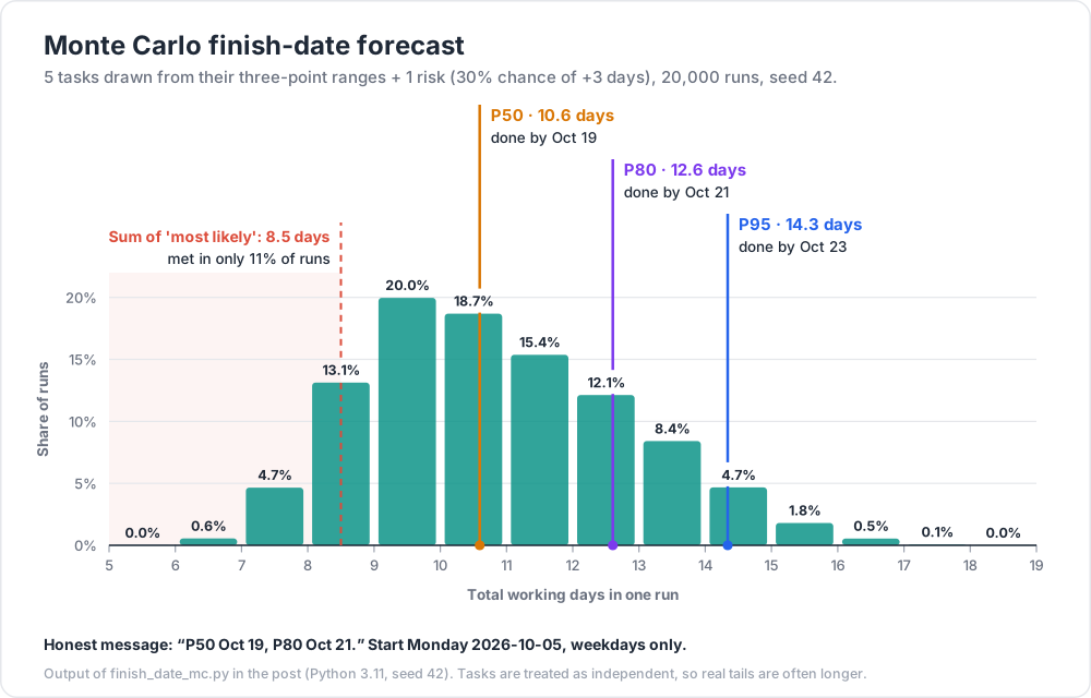
Sum of 'most likely' values: 8.5 days
P50: 10.6 working days -> done by 2026-10-19
P80: 12.6 working days -> done by 2026-10-21
P95: 14.3 working days -> done by 2026-10-23
Chance of finishing within the 'most likely' sum: 11%
5-6 0.0%
6-7 0.6%
7-8 ## 4.7%
8-9 ####### 13.1%
9-10 ########### 20.0%
10-11 ########### 18.7%
11-12 ######### 15.4%
12-13 ####### 12.1%
13-14 ##### 8.4%
14-15 ## 4.7%
15-16 # 1.8%
16-17 0.5%
17-18 0.1%
18-19 0.0%
Read it like this: adding up the "most likely" numbers gives 8.5 days, but that total is met only about 11% of the time. An honest message is "P50 Oct 19, P80 Oct 21."
Watch out: the simulation treats tasks as independent. In real life, one cause (a sick week, a bad dependency) often slows many tasks at once, which makes the tail longer. Add shared risks as
RISKSentries, and compare the output with your own history (next chapter).
Trick:
random.triangular(low, high, mode)is a simpler choice than PERT — note the argument order. It gives more weight to the extremes, so it produces a wider, more cautious range.
Chapter 6 — Track estimate vs actual
You cannot get better at what you do not measure. Keep a tiny log — a CSV is enough — and look at the ratio actual ÷ estimate:
1
2
3
4
5
6
7
8
9
10
11
12
13
14
15
16
17
18
19
20
# calibrate.py — how far off are my estimates?
import csv
import io
import statistics
LOG = """task,estimate_days,actual_days
Login page,2,3
Password reset,1,1.5
CSV export,3,5
Search filter,2,2
Audit log,4,7
Rate limiter,1,1
"""
rows = list(csv.DictReader(io.StringIO(LOG)))
ratios = [float(r["actual_days"]) / float(r["estimate_days"]) for r in rows]
print("ratios:", [round(x, 2) for x in ratios]) # [1.5, 1.5, 1.67, 1.0, 1.75, 1.0]
print("median:", statistics.median(ratios)) # 1.5
print("on time or early:", sum(r <= 1 for r in ratios), "of", len(ratios)) # 2 of 6
A median ratio of 1.5 means: multiply your gut estimate by 1.5 as a first correction. This is reference-class forecasting on your own data. After 20-30 tasks, the spread of ratios is also a good guide for your range.
Chapter 7 — Communicating estimates
Keep estimate, target and commitment apart
McConnell's Software Estimation: Demystifying the Black Art (2006) separates three things that people often mix up:
- an estimate is a prediction ("P80 is 13 days");
- a target is a business wish ("we want it before the conference");
- a commitment is a promise ("we will ship the core flow by Oct 21").
When a target is shorter than the estimate, do not shrink the estimate. Change the scope, the people, or the date — and say which.
A good estimate message
- The range and its confidence: "P50 Oct 19, P80 Oct 21."
- The assumptions: "Assumes the email provider approves us by Friday; excludes the admin screen."
- The biggest risks: "Email approval (30% chance of +3 days)."
- When you will update it: "I will re-estimate after the spike on Wednesday."
Re-estimate when the facts change
An estimate is a forecast, not a vow. When scope grows or a risk happens, update the range at once and say why. Bad news early is useful; bad news on the due date is not.
Story points vs hours
Story points are a team convention, not a law. The 2020 Scrum Guide does not mention story points at all; it only says the Developers who will do the work are responsible for sizing it. Ron Jeffries, who says he may have invented story points, wrote in 2019 that "if I did, I'm sorry now". He explains they started as "ideal days" and recommends slicing stories small instead. Use points or hours as your team prefers — the ideas in this post (breakdown, ranges, tracking actuals) work the same with both.
Practice Exercises
Exercise 1 — One PERT estimate
A task has O = 2, M = 3, P = 10 days. Compute E and SD. Why is E so far above M?
Solution
E = (2 + 4 × 3 + 10) / 6 = 24 / 6 = 4.0 days. SD = (10 − 2) / 6 ≈ 1.33 days. The pessimistic value is 7 days above M but the optimistic is only 1 day below, so the long right tail pulls the mean up.
Exercise 2 — Add up three tasks
Tasks (O, M, P): A (1, 2, 3), B (2, 3, 7), C (1, 1, 4). Give the total expected days, the total SD (assume independence), and a rough P80.
Solution
E: A = 12/6 = 2.0, B = 21/6 = 3.5, C = 9/6 = 1.5. Total 7.0 days.
SD: A = 0.33, B = 0.83, C = 0.5. Total = sqrt(0.111 + 0.694 + 0.25) = sqrt(1.055) ≈ 1.03 days.
Rough P80 = 7.0 + 0.84 × 1.03 ≈ 7.9 days, so "about 8 days, 80% confident".
Exercise 3 — Use your own history
Your log shows a median actual/estimate ratio of 1.5, with 80% of ratios at or below 1.9. Your gut says a new task takes 6 days. What range do you give?
Solution
Median: 6 × 1.5 = 9 days. 80% level: 6 × 1.9 ≈ 11.4 days. Say "about 9 days, 80% confident within 12", and state the assumptions.
Exercise 4 — Break it down
Break "Add CSV export to the orders page" into tasks of one day or less. Include the work people forget.
Solution
One possible list: define columns and format with the product owner (0.25 d); backend endpoint that streams rows (1 d); handle large exports — paging or a background job (1 d); encoding — UTF-8 with BOM if users open it in Excel (0.25 d, see Dev Essentials 01 · Text Encoding); date and number formats (0.25 d); UI button, loading state, errors (0.5 d); permission check (0.25 d); tests (0.5 d); review fixes, docs, deploy (0.5 d). Total ≈ 4.5 days before buffer.
Exercise 5 — Add a risk to the simulation
Add ("Security review asks for changes", 0.20, 2.0) to RISKS and run the script again. What happens to P50 and P80?
Solution
With seed 42 the output becomes P50 ≈ 11.0 and P80 ≈ 13.0 working days (was 10.6 and 12.6), and the chance of meeting the "most likely" sum drops to about 9%. A 20% chance of 2 extra days adds about 0.4 days on average, but it also widens the tail.
Exercise 6 — Rewrite the message
Rewrite this status update: "It'll be done Friday."
Solution
"Most likely Thursday (P50); 80% confident by next Tuesday. This assumes the payments sandbox is back up tomorrow and excludes the refund screen. Biggest risk: the provider's webhook format — I am running a half-day spike on it today and will update the estimate tomorrow noon."
Cheat-sheet
| Idea | Rule of thumb |
|---|---|
| Planning fallacy | Gut estimates are optimistic — even "worst case" ones (Buehler et al., 1994) |
| Hofstadter's law | An aphorism: knowing the bias does not remove it |
| Cone of uncertainty | A model: ~0.25×-4× at concept stage; narrows only as decisions remove uncertainty |
| Breakdown | Split until each task ≤ 1 day with a clear "done" |
| Forgotten work | Integration, tests, review, docs, deploy, migrations, meetings |
| PERT | E = (O + 4M + P) / 6, SD ≈ (P − O) / 6 |
| Summing | Means add; variances add (if independent); SDs do not add |
| Ranges | Say P50 / P80 / P95, not one date |
| Outside view | Compare with similar past work; use your actual/estimate ratio |
| Spike | Time-boxed experiment before estimating an unknown |
| Buffer | One visible project-level line, not hidden padding |
| Monte Carlo | Sample each task 10,000+ times; read percentiles |
| Communicate | Range + confidence + assumptions + risks + next update |
| Estimate ≠ target ≠ commitment | Change scope/people/date, not the estimate |
| Story points | A team convention; not required by the Scrum Guide |
What's next
Dev Essentials 22 · Design Docs covers how to write design docs, ADRs and READMEs that people actually read — the place where your estimate, its assumptions and its risks should be written down.
References
- Kahneman & Tversky (1979) — Intuitive Prediction: Biases and Corrective Procedures (DTIC report)
- Buehler, Griffin & Ross (1994) — Exploring the "planning fallacy", JPSP 67(3) (PDF)
- Flyvbjerg (2006) — From Nobel Prize to Project Management: Getting Risks Right (arXiv copy)
- Construx (Steve McConnell) — The Cone of Uncertainty
- Todd Little (2006) — Schedule estimation and uncertainty surrounding the cone of uncertainty, IEEE Software 23(3)
- McConnell — What Is an "Estimate"? (excerpt from Software Estimation)
- The 2020 Scrum Guide
- Ron Jeffries — Story Points Revisited (2019)
- Python docs — random.betavariate, random.triangular
- Python docs — statistics.quantiles
Note: this post is in progress. Planned additions: a worked example with correlated risks, a spreadsheet version of the Monte Carlo for non-programmers, and forecasting from throughput (tasks per week) instead of estimates.