Real Analysis — 04 · The Riemann Integral

"The area under the curve" is a picture, not a definition. This post turns it into one. You trap the area between an upper sum that overestimates it and a lower sum that underestimates it, and call the function integrable when the trap can be closed as tightly as you like. From that single idea come proofs that every continuous function and every monotone function is integrable, a function that is not integrable (the Dirichlet function), a surprising one that is (Thomae's function), and both halves of the Fundamental Theorem of Calculus, the result that links this post to the derivatives of post 03. The post ends with improper integrals, Lebesgue's exact criterion for Riemann integrability, and the reason a better integral had to be invented.

Series map: 00 The Real Numbers & Completeness → 01 Sequences & Series → 02 Topology of ℝ & Continuity → 03 Differentiation & Taylor's Theorem → 04 The Riemann Integral (this post) → 05 Uniform Convergence & Power Series.

---

Learning Outcome

• Define partitions, upper and lower Darboux sums, and the upper and lower integrals of a bounded function.
• Prove the refinement lemma and deduce that every lower sum is at most every upper sum.
• State and prove the Riemann criterion: $f$ is integrable if and only if $U(f,P) - L(f,P)$ can be made smaller than any $\varepsilon > 0$.
• Compute $\int_0^1 x^2\,dx$ from the definition, with exact upper and lower sums.
• Prove that continuous functions and monotone functions on $[a, b]$ are integrable.
• Show that the Dirichlet function is not integrable and that Thomae's function is integrable with integral $0$.
• Prove linearity, monotonicity and the triangle inequality for integrals.
• State and prove both parts of the Fundamental Theorem of Calculus, and use integration by parts and substitution.
• Decide convergence of the improper integrals $\int_1^\infty x^{-p}\,dx$ and $\int_0^1 x^{-p}\,dx$.
• State Lebesgue's criterion and explain why the Lebesgue integral exists.

---

Chapter 1 — Partitions and Darboux sums

Terminology

• Bounded function — throughout, $f : [a, b] \to \mathbb{R}$ with $a < b$ and $\lvert f(x)\rvert \leq B$ for all $x$. Riemann integration is only defined for bounded functions on closed, bounded intervals; everything else is handled by improper integrals (Chapter 6).
• Partition — a finite set $P = \{x_0, x_1, \dots, x_n\}$ with $a = x_0 < x_1 < \dots < x_n = b$. The $k$-th subinterval is $[x_{k-1}, x_k]$, of length $\Delta x_k = x_k - x_{k-1}$.
• Mesh — the length of the longest subinterval, $\max_k \Delta x_k$.
• Refinement — $Q$ refines $P$ if $P \subseteq Q$ (it keeps every point of $P$ and may add more). The common refinement of $P_1$ and $P_2$ is $P_1 \cup P_2$.
• Local sup and inf — $M_k = \sup\{f(x) : x \in [x_{k-1}, x_k]\}$ and $m_k = \inf\{f(x) : x \in [x_{k-1}, x_k]\}$. These exist because $f$ is bounded (completeness, post 00).
• Upper and lower sums —

$$U(f, P) = \sum_{k=1}^{n} M_k\,\Delta x_k, \qquad L(f, P) = \sum_{k=1}^{n} m_k\,\Delta x_k.$$

Since $m_k \leq M_k$, $L(f, P) \leq U(f, P)$ for every partition. Picture tall rectangles that cover the graph and short rectangles that sit under it.

The refinement lemma

Lemma. If $P \subseteq Q$, then

$$L(f, P) \leq L(f, Q) \leq U(f, Q) \leq U(f, P).$$

Refining can only raise lower sums and lower upper sums.

Proof. By induction it is enough to add one point $z$ to $P$, inside $[x_{k-1}, x_k]$. Only the $k$-th term of the upper sum changes. It is replaced by

$$M'\,(z - x_{k-1}) + M''\,(x_k - z),$$

where $M'$ and $M''$ are the sups of $f$ over $[x_{k-1}, z]$ and $[z, x_k]$. A sup over a smaller set is no bigger, so $M', M'' \leq M_k$, and the new term is at most $M_k(x_k - x_{k-1})$. So $U(f, Q) \leq U(f, P)$. The argument for lower sums is the same with infs, which can only go up. $\blacksquare$

Corollary. For any two partitions $P_1, P_2$: $L(f, P_1) \leq U(f, P_2)$.

Proof. With the common refinement $Q = P_1 \cup P_2$: $L(f, P_1) \leq L(f, Q) \leq U(f, Q) \leq U(f, P_2)$. $\blacksquare$

Upper and lower integrals

Every lower sum is a lower bound for the set of upper sums, so by completeness the following exist and satisfy $L(f,P) \leq \underline{\int} f \leq \overline{\int} f \leq U(f,P)$ for every $P$:

$$\underline{\int_a^b} f = \sup_P L(f, P), \qquad \overline{\int_a^b} f = \inf_P U(f, P).$$

Definition. A bounded $f$ is (Riemann) integrable on $[a, b]$ if $\underline{\int_a^b} f = \overline{\int_a^b} f$. The common value is $\int_a^b f$ or $\int_a^b f(x)\,dx$.

Watch out: this is the Darboux form of the definition. The Riemann-sum form picks a sample point $t_k$ in each subinterval and asks that $\sum f(t_k)\Delta x_k$ tend to a limit as the mesh tends to $0$. The two definitions give the same integrable functions and the same values (Bartle and Sherbert, Section 7.4). The Darboux form is easier to prove things with, because upper and lower sums do not depend on any choice of points.

---

Chapter 2 — The Riemann criterion and a worked example

Theorem (Riemann criterion). A bounded $f$ is integrable on $[a, b]$ if and only if for every $\varepsilon > 0$ there is a partition $P$ with

$$U(f, P) - L(f, P) < \varepsilon.$$

Proof. ($\Leftarrow$) For any such $P$,

$$0 \leq \overline{\int} f - \underline{\int} f \leq U(f, P) - L(f, P) < \varepsilon.$$

The difference is a non-negative number smaller than every $\varepsilon > 0$, so it is $0$.

($\Rightarrow$) Let $I$ be the common value and $\varepsilon > 0$. Since $I = \inf_P U$, there is $P_1$ with $U(f, P_1) < I + \varepsilon/2$. Since $I = \sup_P L$, there is $P_2$ with $L(f, P_2) > I - \varepsilon/2$. For the common refinement $P = P_1 \cup P_2$ the refinement lemma gives

$$U(f, P) - L(f, P) \leq U(f, P_1) - L(f, P_2) < \varepsilon. \qquad \blacksquare$$

The criterion is what you use in practice: you never compute a sup over all partitions, you exhibit one good partition for each $\varepsilon$.

Worked example: the integral of x squared on [0, 1]

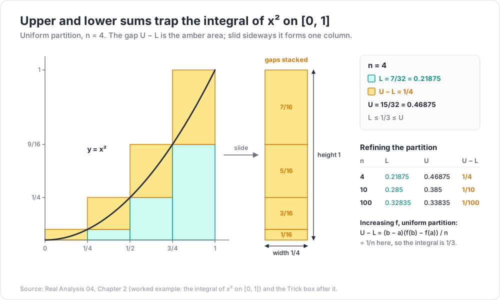
Let $f(x) = x^2$ and let $P_n$ be the uniform partition $x_k = k/n$, $k = 0, \dots, n$, so every $\Delta x_k = 1/n$. Since $f$ is increasing on $[0, 1]$, on $[x_{k-1}, x_k]$ the inf is at the left end and the sup at the right end:

$$m_k = \left(\frac{k-1}{n}\right)^2, \qquad M_k = \left(\frac{k}{n}\right)^2.$$

Using $\sum_{k=1}^{n} k^2 = \frac{n(n+1)(2n+1)}{6}$:

$$U(f, P_n) = \frac{1}{n^3}\sum_{k=1}^{n} k^2 = \frac{(n+1)(2n+1)}{6n^2}, \qquad L(f, P_n) = \frac{1}{n^3}\sum_{k=1}^{n} (k-1)^2 = \frac{(n-1)(2n-1)}{6n^2}.$$

Subtracting,

$$U(f, P_n) - L(f, P_n) = \frac{1}{n^3}\bigl(n^2 - 0^2\bigr) = \frac{1}{n},$$

because the two sums share every term except the largest square $n^2$ and the smallest $0^2$. Given $\varepsilon > 0$, any $n > 1/\varepsilon$ works, so $f$ is integrable. Both sums tend to $\frac{2}{6} = \frac13$, and $L(f, P_n) \leq \int_0^1 x^2\,dx \leq U(f, P_n)$ for every $n$, so

$$\int_0^1 x^2\,dx = \frac13.$$

$n$	$L(f, P_n)$	$U(f, P_n)$	$U - L$
4	$7/32 = 0.21875$	$15/32 = 0.46875$	$1/4$
10	$57/200 = 0.285$	$77/200 = 0.385$	$1/10$
100	$0.32835$	$0.33835$	$1/100$

Trick: for an increasing function on a uniform partition, the gap rectangles stack into a single column of width $\frac{b-a}{n}$ and height $f(b) - f(a)$. So $U - L = \frac{(f(b) - f(a))(b - a)}{n}$ at once. That is the whole proof of the next chapter's monotone theorem.

---

Chapter 3 — Which functions are integrable?

Monotone functions

Theorem. If $f$ is monotone on $[a, b]$, then $f$ is integrable.

Proof. Say $f$ is increasing (it is then bounded by $f(a)$ and $f(b)$). On the uniform partition $P_n$, $M_k = f(x_k)$ and $m_k = f(x_{k-1})$, so the sum telescopes:

$$U(f, P_n) - L(f, P_n) = \frac{b - a}{n}\sum_{k=1}^{n}\bigl(f(x_k) - f(x_{k-1})\bigr) = \frac{(b - a)\bigl(f(b) - f(a)\bigr)}{n}.$$

This is smaller than any given $\varepsilon$ once $n$ is large. $\blacksquare$

A monotone function may have infinitely many jumps (for instance one at every $1/k$), and it is still integrable.

Continuous functions

Theorem. If $f$ is continuous on $[a, b]$, then $f$ is integrable.

Proof. A continuous function on the compact set $[a, b]$ is bounded (EVT) and uniformly continuous (post 02). Let $\varepsilon > 0$. Choose $\delta > 0$ such that $\lvert x - y\rvert < \delta$ implies $\lvert f(x) - f(y)\rvert < \frac{\varepsilon}{b - a}$. Take any partition $P$ with mesh $< \delta$. On each subinterval, $f$ attains its max and min (EVT again) at points $s_k, t_k$ with $\lvert s_k - t_k\rvert < \delta$, so $M_k - m_k = f(s_k) - f(t_k) < \frac{\varepsilon}{b - a}$. Therefore

$$U(f, P) - L(f, P) = \sum_{k=1}^{n} (M_k - m_k)\,\Delta x_k < \frac{\varepsilon}{b - a}\sum_{k=1}^{n} \Delta x_k = \varepsilon. \qquad \blacksquare$$

Common pitfall: plain continuity is not enough for this proof. You need one $\delta$ that works on every subinterval at once, which is exactly uniform continuity. That is why the theorem is stated on a closed, bounded interval.

Finitely many discontinuities

Theorem. If $f$ is bounded on $[a, b]$ and continuous except at finitely many points, then $f$ is integrable.

Sketch. Say $\lvert f\rvert \leq B$ and the bad points are $c_1, \dots, c_m$. Put a small interval of length $\eta$ around each $c_j$. Their total contribution to $U - L$ is at most $2B \cdot m\eta$, which is small when $\eta$ is. On the remaining closed intervals $f$ is continuous, so the previous theorem makes their contribution as small as you like. $\blacksquare$

Changing a function at finitely many points does not change whether it is integrable, or the value of the integral.

A function that is not integrable: Dirichlet

Let $D(x) = 1$ if $x \in \mathbb{Q}$ and $D(x) = 0$ otherwise, on $[0, 1]$. Every subinterval of positive length contains both rationals and irrationals (density of $\mathbb{Q}$ and of the irrationals, post 00), so $M_k = 1$ and $m_k = 0$ for every $k$ and every partition. Therefore $U(D, P) = 1$ and $L(D, P) = 0$ always, the upper integral is $1$, the lower integral is $0$, and $D$ is not Riemann integrable.

A function that is integrable: Thomae

Thomae's function on $[0, 1]$ is

$$T(x) = \begin{cases} 1/q & \text{if } x = p/q \text{ in lowest terms with } q \geq 1, \\ 0 & \text{if } x \text{ is irrational}, \end{cases}$$

with $T(0) = 1$ (as $0 = 0/1$). It is continuous at every irrational and discontinuous at every rational (post 02). Even so:

Claim. $T$ is integrable on $[0, 1]$ and $\int_0^1 T = 0$.

Proof. Every subinterval contains an irrational, so $m_k = 0$ and $L(T, P) = 0$ for every $P$. Let $\varepsilon > 0$. The points where $T(x) \geq \varepsilon/2$ are the fractions $p/q$ with $q \leq 2/\varepsilon$; there are finitely many, say $N$. Choose a partition in which each of these $N$ points lies in subintervals of total length less than $\varepsilon/2$ (for example, give each point its own interval of length less than $\frac{\varepsilon}{4N}$; a point on a boundary touches at most two). On those subintervals $M_k \leq 1$, contributing less than $\varepsilon/2$. On all other subintervals $M_k < \varepsilon/2$, contributing at most $\frac{\varepsilon}{2}\cdot 1$. So $U(T, P) < \varepsilon$. By the Riemann criterion $T$ is integrable, and since every lower sum is $0$, the integral is $0$. $\blacksquare$

For a feel of the numbers: with $\varepsilon = \frac15$, the points where $T \geq \frac1{10}$ are the fractions in $[0, 1]$ with denominator at most $10$, and there are exactly $33$ of them.

---

Chapter 4 — Properties of the integral

Let $f, g$ be integrable on $[a, b]$ and $k \in \mathbb{R}$.

Property	Statement
Linearity	$f + g$ and $kf$ are integrable; $\int (f + g) = \int f + \int g$ and $\int kf = k\int f$
Monotonicity	if $f \leq g$ on $[a, b]$ then $\int_a^b f \leq \int_a^b g$
Additivity	for $a < c < b$: $f$ integrable on $[a, b]$ iff integrable on $[a, c]$ and $[c, b]$, and $\int_a^b f = \int_a^c f + \int_c^b f$
Triangle inequality	$\lvert f\rvert$ is integrable and $\lvert \int_a^b f\rvert \leq \int_a^b \lvert f\rvert$
Bound	if $m \leq f \leq M$ then $m(b - a) \leq \int_a^b f \leq M(b - a)$
Products	$fg$ is integrable

Proof of the sum rule. On any subinterval, $\sup(f + g) \leq \sup f + \sup g$ and $\inf(f + g) \geq \inf f + \inf g$. So $U(f + g, P) \leq U(f, P) + U(g, P)$ and $L(f + g, P) \geq L(f, P) + L(g, P)$. Given $\varepsilon$, take a common refinement where both $U - L$ gaps are below $\varepsilon/2$; then the gap for $f + g$ is below $\varepsilon$, and its integral is squeezed between $L(f,P) + L(g,P)$ and $U(f,P) + U(g,P)$, which both lie within $\varepsilon$ of $\int f + \int g$. $\blacksquare$

Proof of monotonicity. $g - f \geq 0$ has every lower sum $\geq 0$, so $\int (g - f) \geq 0$; then use linearity. $\blacksquare$

Proof of the triangle inequality. On any subinterval, for $x, y$ in it, $\bigl\lvert \lvert f(x)\rvert - \lvert f(y)\rvert \bigr\rvert \leq \lvert f(x) - f(y)\rvert$, so the oscillation $\sup\lvert f\rvert - \inf\lvert f\rvert$ is at most $M_k - m_k$. Hence $U(\lvert f\rvert, P) - L(\lvert f\rvert, P) \leq U(f, P) - L(f, P)$ and $\lvert f\rvert$ is integrable. Since $-\lvert f\rvert \leq f \leq \lvert f\rvert$, monotonicity gives $-\int\lvert f\rvert \leq \int f \leq \int \lvert f\rvert$. $\blacksquare$

Convention. Define $\int_b^a f = -\int_a^b f$ and $\int_a^a f = 0$. Then the additivity formula holds for any order of $a, b, c$.

Mean Value Theorem for integrals. If $f$ is continuous on $[a, b]$, there is $c \in [a, b]$ with $\int_a^b f = f(c)(b - a)$.

Proof. With $m, M$ the min and max of $f$ (EVT), the bound property gives $m \leq \frac{1}{b-a}\int_a^b f \leq M$, and the IVT gives a $c$ where $f$ takes this average value. $\blacksquare$

For example, $\int_0^2 x^2\,dx = \frac83$, so $c^2 \cdot 2 = \frac83$, $c = \frac{2}{\sqrt 3}$: the same point as the MVT example for $x^3$ in post 03, and that is no coincidence, because $\frac{x^3}{3}$ is an antiderivative of $x^2$.

---

Chapter 5 — The Fundamental Theorem of Calculus

Part 1: integrating then differentiating

Theorem (FTC, part 1). Let $f$ be integrable on $[a, b]$ and define

$$F(x) = \int_a^x f(t)\,dt, \qquad x \in [a, b].$$

Then $F$ is continuous on $[a, b]$ (in fact Lipschitz). If $f$ is continuous at $c \in [a, b]$, then $F$ is differentiable at $c$ and $F'(c) = f(c)$ (one-sided at an endpoint).

Proof. Let $\lvert f\rvert \leq B$. For $x < y$, additivity and the bound give $\lvert F(y) - F(x)\rvert = \left\lvert \int_x^y f\right\rvert \leq B(y - x)$. So $F$ is Lipschitz, hence continuous.

Now let $f$ be continuous at $c$ and $\varepsilon > 0$. Choose $\delta$ with $\lvert f(t) - f(c)\rvert < \varepsilon$ for $\lvert t - c\rvert < \delta$. For $0 < \lvert x - c\rvert < \delta$,

$$\frac{F(x) - F(c)}{x - c} - f(c) = \frac{1}{x - c}\int_c^x \bigl(f(t) - f(c)\bigr)\,dt,$$

and the right side has absolute value at most $\frac{1}{\lvert x - c\rvert}\cdot \varepsilon \lvert x - c\rvert = \varepsilon$. $\blacksquare$

So every continuous function has an antiderivative. One famous use: define $\ln x = \int_1^x \frac{dt}{t}$ for $x > 0$. Then FTC 1 gives $\ln'(x) = \frac1x$ at once.

Worked example. Let $G(x) = \int_0^{x^2} \cos(t^2)\,dt$. With $F(u) = \int_0^{u} \cos(t^2)\,dt$, FTC 1 gives $F'(u) = \cos(u^2)$, and $G(x) = F(x^2)$. By the chain rule (post 03),

$$G'(x) = \cos\bigl((x^2)^2\bigr)\cdot 2x = 2x\cos(x^4).$$

Part 2: differentiating then integrating

Theorem (FTC, part 2). Let $F$ be differentiable on $[a, b]$ (one-sided at the endpoints) and suppose $f = F'$ is integrable on $[a, b]$. Then

$$\int_a^b f = F(b) - F(a).$$

Proof. Take any partition $P$. Apply the Mean Value Theorem (post 03) to $F$ on each $[x_{k-1}, x_k]$: there is $t_k$ in the open subinterval with $F(x_k) - F(x_{k-1}) = F'(t_k)\Delta x_k = f(t_k)\Delta x_k$. Summing, the left side telescopes:

$$F(b) - F(a) = \sum_{k=1}^{n} f(t_k)\,\Delta x_k.$$

Since $m_k \leq f(t_k) \leq M_k$, this gives $L(f, P) \leq F(b) - F(a) \leq U(f, P)$ for every $P$. So $F(b) - F(a)$ lies between the lower and upper integrals, which are equal. $\blacksquare$

Watch out: the hypothesis "$F'$ is integrable" cannot be dropped. $F(x) = x^2\sin(1/x^2)$ with $F(0) = 0$ is differentiable on $[-1, 1]$, but $F'(x) = 2x\sin(1/x^2) - \frac{2}{x}\cos(1/x^2)$ for $x \neq 0$ is unbounded near $0$, so it is not Riemann integrable. A derivative can even be bounded and still not Riemann integrable (Volterra's function, 1881).

Integration by parts and substitution

Integration by parts. If $u, v$ are differentiable on $[a, b]$ and $u', v'$ are integrable, then

$$\int_a^b u\,v' = u(b)v(b) - u(a)v(a) - \int_a^b u'\,v.$$

This is FTC 2 applied to $(uv)' = u'v + uv'$. Example: $\int_0^1 x e^x\,dx = \bigl[x e^x\bigr]_0^1 - \int_0^1 e^x\,dx = e - (e - 1) = 1$.

Substitution. If $\varphi : [a, b] \to \mathbb{R}$ is continuously differentiable and $f$ is continuous on an interval containing $\varphi([a, b])$, then

$$\int_a^b f(\varphi(t))\,\varphi'(t)\,dt = \int_{\varphi(a)}^{\varphi(b)} f(u)\,du.$$

Proof: both sides, as functions of the upper limit $b$, have the same derivative (FTC 1 and the chain rule) and agree when $b = a$. Example: with $u = x^2 + 1$, $\int_0^1 2x(x^2 + 1)^3\,dx = \int_1^2 u^3\,du = \frac{2^4 - 1^4}{4} = \frac{15}{4}$.

---

Chapter 6 — Improper integrals

The Riemann integral needs a bounded function on a closed, bounded interval. An improper integral relaxes one of these by a limit.

• Unbounded interval. If $f$ is integrable on $[a, R]$ for every $R > a$, define $\int_a^\infty f = \lim_{R \to \infty} \int_a^R f$ when the limit exists (the integral converges).
• Unbounded function. If $f$ is integrable on $[a + \eta, b]$ for every small $\eta > 0$, define $\int_a^b f = \lim_{\eta \to 0^+} \int_{a+\eta}^b f$.

The p-test. For $p > 0$:

$$\int_1^R x^{-p}\,dx = \begin{cases} \dfrac{1 - R^{1-p}}{p - 1} & p \neq 1, \\ \ln R & p = 1. \end{cases}$$

As $R \to \infty$: if $p > 1$ then $R^{1-p} \to 0$ and the integral converges to $\frac{1}{p - 1}$; if $p \leq 1$ it diverges to $\infty$. Near $0$ the roles swap: $\int_0^1 x^{-p}\,dx$ converges (to $\frac{1}{1 - p}$) exactly when $p < 1$.

Integral	Converges?	Value
$\int_1^\infty x^{-2}\,dx$	yes ($p = 2 > 1$)	$1$
$\int_1^\infty x^{-1}\,dx$	no ($p = 1$)	diverges
$\int_0^1 x^{-1/2}\,dx$	yes ($p = \frac12 < 1$)	$2$
$\int_0^\infty e^{-x}\,dx$	yes	$1$

This mirrors the $p$-series test of post 01: $\sum 1/k^p$ converges exactly when $p > 1$. The integral test makes the link precise: for $f$ positive and decreasing on $[1, \infty)$, $\sum f(k)$ and $\int_1^\infty f$ converge or diverge together.

Common pitfall: $\int_{-\infty}^{\infty} f$ is defined as $\int_{-\infty}^0 f + \int_0^\infty f$ with both limits existing separately. $\lim_{R \to \infty}\int_{-R}^{R} x\,dx = 0$, but $\int_{-\infty}^\infty x\,dx$ diverges.

---

Chapter 7 — Lebesgue's criterion, and why Lebesgue integration exists

Measure zero

A set $A \subseteq \mathbb{R}$ has measure zero if for every $\varepsilon > 0$ it can be covered by countably many open intervals whose total length is less than $\varepsilon$.

• Every finite set has measure zero.
• Every countable set $\{a_1, a_2, \dots\}$ has measure zero: cover $a_k$ by an interval of length $\varepsilon/2^{k+1}$; the total is at most $\varepsilon/2$. So $\mathbb{Q}$ has measure zero (it is countable, post 00).
• An interval $[c, d]$ with $c < d$ does not have measure zero.

Theorem (Lebesgue's criterion). A function $f : [a, b] \to \mathbb{R}$ is Riemann integrable if and only if $f$ is bounded and the set of points where $f$ is discontinuous has measure zero.

This explains every example in the post at once:

Function	Discontinuities	Integrable?
continuous $f$	none	yes
monotone $f$	countable (jumps)	yes
Thomae $T$	the rationals: countable	yes
Dirichlet $D$	every point of $[0, 1]$	no
$x^{-1/2}$ on $(0, 1]$	— but unbounded	not Riemann; only improper

The proof is in Abbott, Section 7.6, and Rudin, Theorem 11.33.

Why a better integral was needed

The Riemann integral does not behave well under limits. Enumerate the rationals in $[0, 1]$ as $q_1, q_2, \dots$ and let $f_n$ be $1$ at $q_1, \dots, q_n$ and $0$ elsewhere. Each $f_n$ has finitely many discontinuities, so it is integrable with $\int_0^1 f_n = 0$. The functions increase and are bounded by $1$, and $f_n(x) \to D(x)$ at every $x$. But the limit $D$ is not Riemann integrable, so "$\int f_n \to \int \lim f_n$" is not even meaningful.

Lebesgue's integral (1902) partitions the range of $f$ instead of its domain, and measures the sets where $f$ takes values in each range slice. It integrates $D$ (answer $0$, since $\mathbb{Q}$ has measure zero), agrees with the Riemann integral whenever the latter exists, and satisfies clean limit theorems such as the Monotone and Dominated Convergence Theorems. Post 05 shows the Riemann-world substitute: limits and integrals commute when convergence is uniform.

---

Practice Exercises

Exercise 1. For $f(x) = x$ on $[0, 1]$ and the uniform partition $P_n$, compute $U(f, P_n)$ and $L(f, P_n)$ and deduce $\int_0^1 x\,dx$.

Solution

$M_k = k/n$ and $m_k = (k-1)/n$, each times $\Delta x_k = 1/n$. With $\sum_{k=1}^n k = \frac{n(n+1)}{2}$: $U = \frac{n+1}{2n}$ and $L = \frac{n-1}{2n}$. So $U - L = \frac1n \to 0$ and both tend to $\frac12$. Hence $\int_0^1 x\,dx = \frac12$.

Exercise 2. For $f(x) = x^3$ on $[0, 2]$ with the uniform partition into $n$ pieces, show $U - L = \frac{16}{n}$. How large must $n$ be for $U - L < 0.01$?

Solution

By the trick of Chapter 2 (increasing function, uniform partition), $U - L = \frac{(b - a)(f(b) - f(a))}{n} = \frac{2 \cdot 8}{n} = \frac{16}{n}$. Explicitly, $U = \frac{4(n+1)^2}{n^2}$ and $L = \frac{4(n-1)^2}{n^2}$, whose difference is $\frac{16n}{n^2}$. Then $\frac{16}{n} < 0.01$ needs $n > 1600$, so $n = 1601$ is the smallest. Both sums tend to $4 = \int_0^2 x^3\,dx$.

Exercise 3. Let $f = 0$ on $[0, 1]$ except $f(\frac12) = 5$. Prove from the definition that $f$ is integrable with integral $0$.

Solution

Every lower sum is $0$ (each subinterval contains points where $f = 0$). Given $\varepsilon > 0$, take $0 < \delta < \min(\frac{\varepsilon}{10}, \frac12)$ and the partition $\{0, \frac12 - \delta, \frac12 + \delta, 1\}$. Only the middle subinterval has $M_k = 5$, so $U = 5 \cdot 2\delta < \varepsilon$. By the Riemann criterion $f$ is integrable, and the integral is squeezed to $0$.

Exercise 4. Evaluate $\int_0^1 \frac{dx}{\sqrt x}$ and decide whether $\int_1^\infty \frac{dx}{x}$ converges.

Solution

$\int_\eta^1 x^{-1/2}\,dx = 2 - 2\sqrt\eta \to 2$ as $\eta \to 0^+$, so the first integral is $2$. For the second, $\int_1^R \frac{dx}{x} = \ln R \to \infty$: it diverges ($p = 1$).

Exercise 5. Let $f$ be continuous on $[a, b]$ with $f \geq 0$ and $\int_a^b f = 0$. Prove $f(x) = 0$ for all $x$.

Solution

Suppose $f(c) > 0$ for some $c$. By continuity there is an interval $[c', d'] \subseteq [a, b]$ of positive length containing $c$ on which $f \geq \frac{f(c)}{2}$. By additivity and monotonicity, $\int_a^b f \geq \int_{c'}^{d'} f \geq \frac{f(c)}{2}(d' - c') > 0$. Contradiction. (Continuity is needed: Thomae's function is $\geq 0$, not identically $0$, and has integral $0$.)

Exercise 6. Find $H'(x)$ for $H(x) = \int_{x}^{x^2} \frac{dt}{t}$ on $x > 0$, and explain the answer.

Solution

Write $H(x) = \int_1^{x^2} \frac{dt}{t} - \int_1^{x} \frac{dt}{t}$. By FTC 1 and the chain rule, $H'(x) = \frac{1}{x^2}\cdot 2x - \frac1x = \frac1x$. Indeed $H(x) = \ln(x^2) - \ln x = \ln x$.

Exercise 7. Explain why the pointwise limit of integrable functions need not be integrable, using the functions $f_n$ from Chapter 7.

Solution

Each $f_n$ is $1$ at $n$ rationals and $0$ elsewhere, so it has $n$ discontinuities and $\int_0^1 f_n = 0$. At a rational $x = q_m$, $f_n(x) = 1$ once $n \geq m$; at an irrational $x$, $f_n(x) = 0$ for all $n$. So $f_n \to D$ pointwise, and $D$ is not Riemann integrable (upper integral 1, lower integral 0). The convergence is not uniform: $\sup\lvert f_n - D\rvert = 1$ for every $n$.

---

Cheat-sheet

Idea	Statement
Upper / lower sum	$U = \sum M_k\Delta x_k$, $L = \sum m_k\Delta x_k$
Refinement	$P \subseteq Q \Rightarrow L(P) \leq L(Q) \leq U(Q) \leq U(P)$
Integrable	lower integral $=$ upper integral
Riemann criterion	for every $\varepsilon$ some $P$ has $U - L < \varepsilon$
Increasing, uniform partition	$U - L = (b - a)(f(b) - f(a))/n$
$x^2$ on $[0,1]$	$U - L = 1/n$, integral $1/3$
Always integrable	continuous; monotone; bounded with finitely many discontinuities
Not integrable	Dirichlet (upper 1, lower 0); unbounded functions
Thomae	integrable, integral 0
Triangle inequality	$\lvert \int f\rvert \leq \int \lvert f\rvert$
FTC 1	$F(x) = \int_a^x f$ is Lipschitz; $F'(c) = f(c)$ where $f$ is continuous
FTC 2	$F' = f$ integrable $\Rightarrow \int_a^b f = F(b) - F(a)$
p-test	$\int_1^\infty x^{-p}$ converges iff $p > 1$; $\int_0^1 x^{-p}$ iff $p < 1$
Lebesgue criterion	bounded and discontinuities of measure zero

---

What's next

Post 05 studies sequences and series of functions. It separates pointwise from uniform convergence, proves that uniform limits of continuous functions are continuous and that integrals commute with uniform limits (the theorem the Dirichlet example above was missing), and then applies everything to power series: radius of convergence, term-by-term differentiation and integration, Abel's theorem and the Weierstrass approximation theorem.

---

References

• Stephen Abbott, Understanding Analysis, 2nd ed., Springer (Undergraduate Texts in Mathematics), 2015 — Chapter 7, "The Riemann Integral", including Section 7.6 on Lebesgue's criterion.
• Walter Rudin, Principles of Mathematical Analysis, 3rd ed., McGraw-Hill, 1976 — Chapter 6, "The Riemann–Stieltjes Integral", and Chapter 11 for Lebesgue theory.
• Robert G. Bartle and Donald R. Sherbert, Introduction to Real Analysis, 4th ed., Wiley, 2011 — Chapter 7 (Riemann sums, the Darboux integral and their equivalence, FTC, Lebesgue's criterion).
• Michael Spivak, Calculus, 4th ed., Publish or Perish, 2008 — Chapters 13–14 (integrals and the Fundamental Theorem).
• Jiří Lebl, Basic Analysis I: Introduction to Real Analysis, free textbook — jirka.org/ra, Chapter 5.
• MIT OpenCourseWare, 18.100A Real Analysis (Fall 2020), lecture notes on the Riemann integral and the Fundamental Theorem of Calculus.

Note: this post is in progress. Planned additions: the Riemann–Stieltjes integral, a full proof of Lebesgue's criterion, the integral test with its error bounds, and the integral form of the Taylor remainder from post 03.