Calculus states that a continuous function on a closed interval has a maximum and takes every value in between. Both facts can fail on an open interval or on the rationals, and the reason is not the function but the set it lives on. This post first studies subsets of $\mathbb{R}$ — open, closed and compact sets — and then functions: the $\varepsilon$ – $\delta$ definition of a limit and of continuity, with fully worked $\delta$ 's, the Extreme Value Theorem, the Intermediate Value Theorem, and uniform continuity. It builds directly on the Axiom of Completeness (Real Analysis 00) and on Bolzano–Weierstrass and sequences (Real Analysis 01).

Series map: 00 The Real Numbers & Completeness → 01 Sequences & Series → 02 Topology of ℝ & Continuity (this post) → 03 Differentiation & Taylor's Theorem → 04 The Riemann Integral → 05 Uniform Convergence & Power Series.

Learning Outcome

Define open sets, limit points, closed sets and closure, and decide which of these a given set is.
Define compactness by sequences and by open covers, and prove one direction of the Heine–Borel Theorem.
State the $\varepsilon$ – $\delta$ definition of a functional limit and its sequential criterion, and use the criterion to prove that a limit does not exist.
Prove continuity from the definition, with an explicit $\delta$ for $f(x) = x^2$ at a point, and check it numerically.
Prove that continuous images of compact sets are compact, and deduce the Extreme Value Theorem.
Prove the Intermediate Value Theorem using the supremum.
Define uniform continuity, show that $1/x$ and $x^2$ fail it on suitable domains, and prove that continuous functions on compact sets are uniformly continuous.
Describe the discontinuity sets of the Dirichlet and Thomae functions.

Chapter 1 — Open and closed sets

Terminology

$\varepsilon$ -neighbourhood — $V_\varepsilon(a) = (a - \varepsilon, a + \varepsilon)$ .
Open set — $O \subseteq \mathbb{R}$ is open if for every $a \in O$ there is $\varepsilon > 0$ with $V_\varepsilon(a) \subseteq O$ . Every point has some room around it inside the set.
Limit point of $A$ — a point $x$ (in $A$ or not) such that every $V_\varepsilon(x)$ contains a point of $A$ other than $x$ .
Isolated point of $A$ — a point of $A$ that is not a limit point of $A$ .
Closed set — a set that contains all of its limit points.
Closure — $\overline{A} = A \cup L$ , where $L$ is the set of limit points of $A$ .
Complement — $A^c = \mathbb{R} \setminus A$ .

Examples of open sets

$\mathbb{R}$ and $\emptyset$ are open (the second vacuously).
Every open interval $(a, b)$ is open: for $x \in (a,b)$ take $\varepsilon = \min(x - a,\ b - x)$ ; then $V_\varepsilon(x) \subseteq (a,b)$ .
$[0, 1)$ is not open: no neighbourhood of $0$ fits inside it.

Theorem. (i) Any union of open sets is open. (ii) A finite intersection of open sets is open.

Proof. (i) A point of the union lies in some $O_\lambda$ , and a neighbourhood inside $O_\lambda$ is inside the union. (ii) If $a \in O_1 \cap \cdots \cap O_N$ , choose $\varepsilon_i$ with $V_{\varepsilon_i}(a) \subseteq O_i$ and take $\varepsilon = \min_i \varepsilon_i > 0$ . $\blacksquare$

The word "finite" in (ii) matters: $\bigcap_{n=1}^\infty \left(-\frac1n, \frac1n\right) = \{0\}$ , which is not open. With infinitely many $\varepsilon_i$ the minimum can be $0$ .

Limit points and closed sets

Theorem. $x$ is a limit point of $A$ if and only if $x = \lim a_n$ for some sequence $(a_n)$ in $A$ with $a_n \ne x$ for all $n$ .

Proof. ( $\Rightarrow$ ) For each $n$ pick $a_n \in V_{1/n}(x) \cap A$ with $a_n \ne x$ ; then $\lvert a_n - x \rvert < 1/n \to 0$ . ( $\Leftarrow$ ) Given $\varepsilon$ , the terms $a_n$ with $n$ large lie in $V_\varepsilon(x)$ , are in $A$ , and differ from $x$ . $\blacksquare$

So a set is closed exactly when it contains the limit of every convergent sequence of its points (constant sequences included, for points of $A$ itself).

Set	Limit points	Open?	Closed?
$[a, b]$	$[a, b]$	no	yes
$(a, b)$	$[a, b]$	yes	no
$\{1/n : n \in \mathbb{N}\}$	$\{0\}$	no	no ( $0$ missing)
$\{0\} \cup \{1/n : n \in \mathbb{N}\}$	$\{0\}$	no	yes
$\mathbb{Z}$	none	no	yes (vacuously)
$\mathbb{Q}$	$\mathbb{R}$ (density)	no	no
$\mathbb{R}$ , $\emptyset$	$\mathbb{R}$ , none	yes	yes

Theorem. A set is open if and only if its complement is closed. Consequently, finite unions and arbitrary intersections of closed sets are closed (De Morgan's laws).

Proof of one direction. Let $O$ be open and let $x$ be a limit point of $O^c$ . If $x \in O$ , some $V_\varepsilon(x) \subseteq O$ contains no point of $O^c$ , contradicting that $x$ is a limit point of $O^c$ . So $x \in O^c$ , and $O^c$ is closed. $\blacksquare$

The closure $\overline{A}$ is the smallest closed set containing $A$ ; for example $\overline{\mathbb{Q}} = \mathbb{R}$ and $\overline{(a,b)} = [a,b]$ .

Watch out: "closed" is not the opposite of "open". A set can be both ( $\mathbb{R}$ , $\emptyset$ — the only two such subsets of $\mathbb{R}$ ) or neither ( $[0,1)$ , $\mathbb{Q}$ ).

Chapter 2 — Compact and connected sets

Terminology

Compact (sequential definition) — $K$ is compact if every sequence in $K$ has a subsequence that converges to a limit in $K$ .
Open cover of $A$ — a collection of open sets $\{O_\lambda\}$ whose union contains $A$ . A finite subcover is a finite subcollection that still covers $A$ .
Compact (cover definition) — every open cover of $K$ has a finite subcover.
Bounded set — $\lvert x \rvert \le M$ for all $x$ in the set, for some $M$ .

Heine–Borel

Theorem (Heine–Borel). For $K \subseteq \mathbb{R}$ the following are equivalent:
(i) $K$ is compact (sequential definition);
(ii) $K$ is closed and bounded;
(iii) every open cover of $K$ has a finite subcover.

Proof of (ii) ⇒ (i). Let $(x_n)$ be a sequence in $K$ . It is bounded because $K$ is, so by Bolzano–Weierstrass (Real Analysis 01) it has a convergent subsequence $x_{n_k} \to x$ . Either $x$ equals infinitely many of the $x_{n_k}$ , so $x \in K$ , or it is a limit point of $K$ , and then $x \in K$ because $K$ is closed. $\blacksquare$

Proof of (i) ⇒ (ii). If $K$ were unbounded, choose $x_n \in K$ with $\lvert x_n \rvert > n$ ; no subsequence is bounded, so none converges. If $K$ were not closed, some limit point $x \notin K$ is the limit of a sequence in $K$ ; every subsequence also tends to $x \notin K$ . $\blacksquare$

The equivalence with (iii) takes more work; see Abbott Section 3.3 and Rudin Theorems 2.40–2.41.

Nested compact sets. If $K_1 \supseteq K_2 \supseteq K_3 \supseteq \cdots$ are nonempty compact sets, then $\bigcap_n K_n \ne \emptyset$ . (Pick $x_n \in K_n$ . The sequence lies in $K_1$ , so a subsequence converges to some $x \in K_1$ . For each fixed $m$ , the terms with $n_k \ge m$ lie in the closed set $K_m$ , so $x \in K_m$ .) This generalizes the Nested Interval Property of Real Analysis 00 from intervals to any compact sets.

Examples. $[0,1]$ and the Cantor set (an intersection of closed sets, inside $[0,1]$ ) are compact. $(0,1)$ is not: the sequence $1/n$ has every subsequence tending to $0 \notin (0,1)$ . Equivalently, the open cover $\{(1/n, 1) : n \ge 2\}$ of $(0,1)$ has no finite subcover, since the union of finitely many of these sets is $(1/N, 1)$ for the largest $N$ used, which misses $(0, 1/N]$ . $\mathbb{R}$ is closed but not bounded, so not compact.

Trick: use the sequential definition when you have a sequence in hand (most proofs in this post). Use the cover definition to pass from "local" information at each point to a "global" statement with finitely many pieces.

Connected sets

Two nonempty sets $A, B$ are separated if $\overline{A} \cap B = \emptyset$ and $A \cap \overline{B} = \emptyset$ . A set is connected if it is not a union of two separated sets.

Theorem. A set $E \subseteq \mathbb{R}$ is connected if and only if it is an interval: whenever $a < c < b$ with $a, b \in E$ , also $c \in E$ .

$\mathbb{Q}$ is not connected: $\mathbb{Q} = \{r < \sqrt2\} \cup \{r > \sqrt2\}$ splits it into two separated pieces. This gap is exactly why the Intermediate Value Theorem fails for functions on $\mathbb{Q}$ .

Chapter 3 — Limits of functions

Terminology

Functional limit — let $f : A \to \mathbb{R}$ and let $c$ be a limit point of $A$ . Then $\lim_{x \to c} f(x) = L$ means: for every $\varepsilon > 0$ there is $\delta > 0$ such that for all $x \in A$ with $0 < \lvert x - c \rvert < \delta$ , $\lvert f(x) - L \rvert < \varepsilon$ .
The condition $0 < \lvert x - c \rvert$ means the value $f(c)$ (if it exists) plays no role in the limit.

A first example

Claim. $\lim_{x \to 2} (3x + 1) = 7$ .

Proof. $\lvert (3x + 1) - 7 \rvert = 3 \lvert x - 2 \rvert$ . Given $\varepsilon > 0$ , let $\delta = \varepsilon / 3$ . If $0 < \lvert x - 2 \rvert < \delta$ then $\lvert (3x+1) - 7 \rvert < 3\delta = \varepsilon$ . $\blacksquare$

For a linear function, $\delta$ is simply $\varepsilon$ divided by the slope. Nonlinear functions need one extra step (Chapter 4).

The sequential criterion

Theorem. $\lim_{x \to c} f(x) = L$ if and only if for every sequence $(x_n)$ in $A$ with $x_n \ne c$ and $x_n \to c$ , the sequence $f(x_n) \to L$ .

Proof of (⇒). Let $\varepsilon > 0$ and take the $\delta$ from the definition. Since $x_n \to c$ , there is $N$ with $\lvert x_n - c \rvert < \delta$ for $n \ge N$ , and $x_n \ne c$ . So $\lvert f(x_n) - L \rvert < \varepsilon$ for $n \ge N$ . $\blacksquare$

Proof of (⇐). Suppose the limit is not $L$ . Negating the definition (Real Analysis 00): there is $\varepsilon_0 > 0$ such that for every $\delta > 0$ some $x \in A$ has $0 < \lvert x - c \rvert < \delta$ and $\lvert f(x) - L \rvert \ge \varepsilon_0$ . Apply this with $\delta = 1/n$ for each $n$ to get $x_n \ne c$ with $\lvert x_n - c \rvert < 1/n$ , so $x_n \to c$ , but $\lvert f(x_n) - L \rvert \ge \varepsilon_0$ for all $n$ , so $f(x_n) \not\to L$ . $\blacksquare$

The same pattern — negate the $\varepsilon$ – $\delta$ statement, then use $\delta = 1/n$ to build a sequence — proves the sequential criteria for continuity and for uniform continuity below.

Corollary (divergence criterion). If two sequences $x_n \to c$ and $y_n \to c$ (terms $\ne c$ ) have $f(x_n)$ and $f(y_n)$ tending to different limits, then $\lim_{x \to c} f(x)$ does not exist.

Example. $f(x) = \sin(1/x)$ at $c = 0$ . Take $x_n = \frac{1}{2n\pi}$ and $y_n = \frac{1}{2n\pi + \pi/2}$ . Both tend to $0$ , but $\sin(1/x_n) = \sin(2n\pi) = 0$ and $\sin(1/y_n) = \sin(2n\pi + \pi/2) = 1$ for every $n$ . The limit does not exist: the graph oscillates between $-1$ and $1$ infinitely often near $0$ .

Chapter 4 — Continuity

Terminology

Removable discontinuity at $c$ — $\lim_{x \to c} f(x)$ exists but differs from $f(c)$ (or $f(c)$ is undefined).
Jump discontinuity — the one-sided limits $\lim_{x \to c^-} f(x)$ and $\lim_{x \to c^+} f(x)$ both exist but are different.
Essential discontinuity — at least one one-sided limit does not exist, as for $\sin(1/x)$ at $0$ .
Lipschitz function — there is $K \ge 0$ with $\lvert f(x) - f(y) \rvert \le K \lvert x - y \rvert$ for all $x, y$ in the domain.

Definition

$f : A \to \mathbb{R}$ is continuous at $c \in A$ if for every $\varepsilon > 0$ there is $\delta > 0$ such that for all $x \in A$ with $\lvert x - c \rvert < \delta$ , $\lvert f(x) - f(c) \rvert < \varepsilon$ . It is continuous on $A$ if it is continuous at every point of $A$ .

Equivalently (sequential criterion): $f$ is continuous at $c$ if and only if $x_n \to c$ with $x_n \in A$ implies $f(x_n) \to f(c)$ . If $c$ is a limit point of $A$ , this is the same as $\lim_{x \to c} f(x) = f(c)$ . At an isolated point of $A$ every function is continuous.

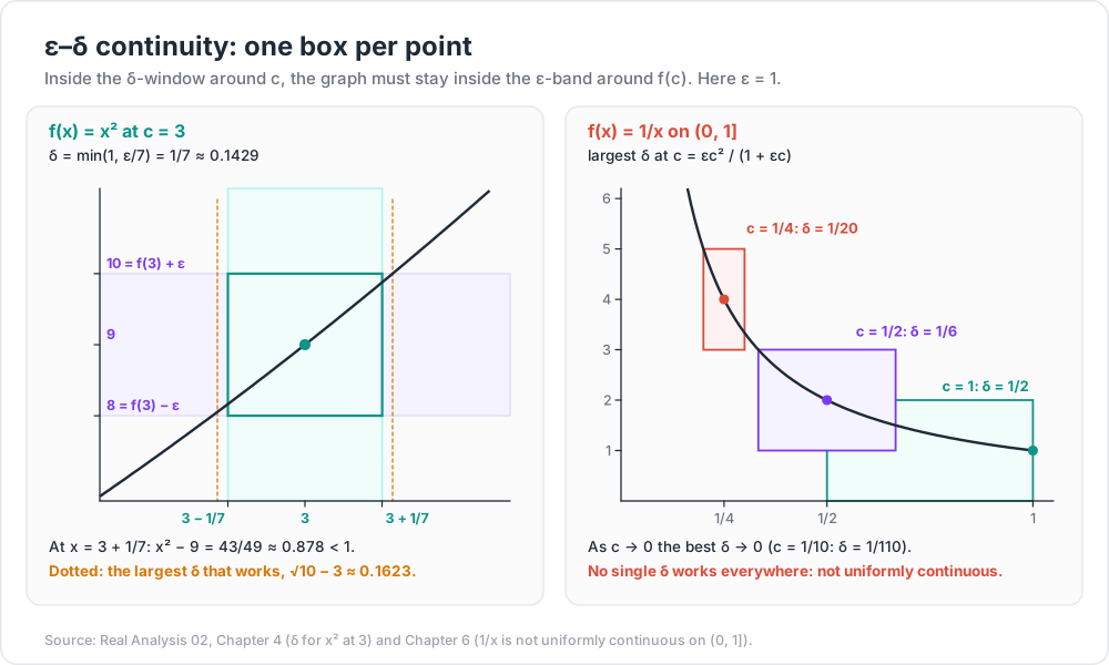
Worked example: a delta for x squared at c = 3

Claim. $f(x) = x^2$ is continuous at $c = 3$ .

Scratch work. Factor: $\lvert x^2 - 9 \rvert = \lvert x - 3 \rvert \, \lvert x + 3 \rvert$ . The factor $\lvert x - 3 \rvert$ is what $\delta$ controls; the factor $\lvert x + 3 \rvert$ must be bounded. Agree in advance that $\delta \le 1$ . Then $\lvert x - 3 \rvert < 1$ gives $2 < x < 4$ , so $\lvert x + 3 \rvert < 7$ , and

$\lvert x^2 - 9 \rvert < 7 \lvert x - 3 \rvert.$

This is less than $\varepsilon$ when $\lvert x - 3 \rvert < \varepsilon / 7$ .

Proof. Let $\varepsilon > 0$ and set $\delta = \min\left(1, \frac{\varepsilon}{7}\right)$ . If $\lvert x - 3 \rvert < \delta$ , then $\lvert x - 3 \rvert < 1$ , so $\lvert x + 3 \rvert < 7$ , and $\lvert x^2 - 9 \rvert < 7 \cdot \frac{\varepsilon}{7} = \varepsilon$ . $\blacksquare$

Checking with numbers. For $\varepsilon = 1$ the rule gives $\delta = \min(1, 1/7) = 1/7 \approx 0.1429$ . The worst case is at the right end, $x = 3 + \tfrac17$ : $x^2 - 9 = \tfrac67 + \tfrac{1}{49} = \tfrac{43}{49} \approx 0.878 < 1$ . At the left end, $9 - (3 - \tfrac17)^2 = \tfrac{41}{49} \approx 0.837 < 1$ . The largest $\delta$ that works is $\sqrt{10} - 3 \approx 0.1623$ ; the proof's $\delta$ is a little smaller, which is fine — any $\delta$ that works is enough.

$\varepsilon$	$\delta = \min(1, \varepsilon/7)$	worst $\lvert x^2 - 9\rvert$ at $x = 3 + \delta$	largest valid $\delta$
$1$	$1/7 \approx 0.1429$	$43/49 \approx 0.8776$	$\sqrt{10} - 3 \approx 0.1623$
$0.1$	$1/70 \approx 0.01429$	$421/4900 \approx 0.08592$	$\sqrt{9.1} - 3 \approx 0.01662$

Trick: the " $\delta = \min(1, \dots)$ " move is the standard way to handle a nonlinear factor: first restrict $x$ to a fixed interval around $c$ to bound the awkward factor by a constant, then divide $\varepsilon$ by that constant.

Building continuous functions

Algebraic Continuity Theorem. If $f$ and $g$ are continuous at $c$ , so are $kf$ , $f + g$ , $fg$ , and $f/g$ (if $g(c) \ne 0$ ).

Proof. Use the sequential criterion: if $x_n \to c$ then $f(x_n) \to f(c)$ and $g(x_n) \to g(c)$ , and the Algebraic Limit Theorem (Real Analysis 01) does the rest. $\blacksquare$

Since $f(x) = x$ and constants are continuous, every polynomial is continuous on $\mathbb{R}$ , and every rational function is continuous wherever its denominator is not zero.

Composition. If $g$ is continuous at $c$ and $f$ is continuous at $g(c)$ , then $f \circ g$ is continuous at $c$ .

Proof. Let $\varepsilon > 0$ . Choose $\eta > 0$ with $\lvert y - g(c) \rvert < \eta \Rightarrow \lvert f(y) - f(g(c)) \rvert < \varepsilon$ . Then choose $\delta > 0$ with $\lvert x - c \rvert < \delta \Rightarrow \lvert g(x) - g(c) \rvert < \eta$ . Chaining, $\lvert x - c \rvert < \delta \Rightarrow \lvert f(g(x)) - f(g(c)) \rvert < \varepsilon$ . $\blacksquare$

So $\sqrt{1 + x^2}$ , $\sin(x^3)$ and $e^{\cos x}$ are continuous (given that the square root, sine, cosine and exponential functions are continuous on their domains).

Chapter 5 — Continuous functions on compact sets and intervals

Compactness is preserved

Theorem. If $f : K \to \mathbb{R}$ is continuous and $K$ is compact, then $f(K) = \{f(x) : x \in K\}$ is compact.

Proof. Let $(y_n)$ be a sequence in $f(K)$ ; write $y_n = f(x_n)$ with $x_n \in K$ . By compactness a subsequence $x_{n_k} \to x \in K$ . By continuity $y_{n_k} = f(x_{n_k}) \to f(x) \in f(K)$ . So every sequence in $f(K)$ has a subsequence converging in $f(K)$ . $\blacksquare$

The Extreme Value Theorem

Theorem (EVT). If $f : K \to \mathbb{R}$ is continuous and $K$ is compact and nonempty, then $f$ attains a maximum and a minimum: there are $x_0, x_1 \in K$ with $f(x_0) \le f(x) \le f(x_1)$ for all $x \in K$ .

Proof. $f(K)$ is compact, hence bounded, so $s = \sup f(K)$ exists (Axiom of Completeness). By the $\varepsilon$ -characterization, for each $n$ there is $y_n \in f(K)$ with $s - 1/n < y_n \le s$ , so $y_n \to s$ . Since $f(K)$ is closed, $s \in f(K)$ : $s = f(x_1)$ for some $x_1 \in K$ . The minimum is the same argument with $\inf$ . $\blacksquare$

Every hypothesis is needed:

Function and domain	What fails	Max attained?
$f(x) = x$ on $(0, 1)$	domain not closed	no ( $\sup = 1$ not reached)
$f(x) = x$ on $[0, \infty)$	domain not bounded	no (unbounded)
$f(x) = 1/x$ on $(0, 1]$	domain not closed	no (unbounded)
$f(0) = 0$ , $f(x) = 1 - x$ on $(0, 1]$	$f$ not continuous at $0$	no ( $\sup = 1$ not reached)

The Intermediate Value Theorem

Theorem (IVT). Let $f : [a, b] \to \mathbb{R}$ be continuous, and let $L$ be a number strictly between $f(a)$ and $f(b)$ . Then there is $c \in (a, b)$ with $f(c) = L$ .

Proof (via the supremum). Replacing $f$ by $f - L$ (and by $-f$ if needed), assume $f(a) < 0 < f(b)$ and find $c$ with $f(c) = 0$ . Let

$S = \{x \in [a, b] : f(x) < 0\}.$

$S$ contains $a$ and is bounded above by $b$ , so $c = \sup S$ exists, and $a \le c \le b$ .

$f(c) > 0$ is impossible. By continuity there is $\delta > 0$ with $f(x) > 0$ for $x \in (c - \delta, c]$ (take $\varepsilon = f(c)$ ). Then no point of $S$ lies in $(c - \delta, c]$ , and none lies above $c$ , so $c - \delta$ is an upper bound of $S$ smaller than $c$ . Contradiction.

$f(c) < 0$ is impossible. Then $c \ne b$ since $f(b) > 0$ , and by continuity $f(x) < 0$ on $[c, c + \delta)$ for some $\delta > 0$ (small enough that $c + \delta \le b$ ). So $c + \delta/2 \in S$ , contradicting that $c$ is an upper bound.

Hence $f(c) = 0$ , and $c \ne a, b$ since $f(a) < 0 < f(b)$ . $\blacksquare$

A second proof: $f([a,b])$ is connected (continuous images of connected sets are connected), hence an interval by the theorem in Chapter 2, so it contains every value between $f(a)$ and $f(b)$ . A third uses bisection and the Nested Interval Property — which is also an algorithm.

Worked example. $p(x) = x^3 + x - 1$ has a root in $(0,1)$ , since $p(0) = -1 < 0 < 1 = p(1)$ . Bisection narrows it:

interval	midpoint $m$	$p(m)$	keep
$[0, 1]$	$0.5$	$-0.375$	$[0.5, 1]$
$[0.5, 1]$	$0.75$	$0.171875$	$[0.5, 0.75]$
$[0.5, 0.75]$	$0.625$	$\approx -0.1309$	$[0.625, 0.75]$
$[0.625, 0.75]$	$0.6875$	$\approx 0.01245$	$[0.625, 0.6875]$

The root is $\approx 0.6823$ . (It is the only real root: $p'(x) = 3x^2 + 1 > 0$ , so $p$ is strictly increasing.)

Common pitfall: the IVT says nothing about functions on sets with gaps. On $\mathbb{Q} \cap [0, 2]$ , the continuous function $g(x) = x^2 - 2$ is negative at $0$ and positive at $2$ but has no rational zero.

Chapter 6 — Uniform continuity

Definition

$f : A \to \mathbb{R}$ is uniformly continuous on $A$ if for every $\varepsilon > 0$ there is $\delta > 0$ such that for all $x, y \in A$ with $\lvert x - y \rvert < \delta$ , $\lvert f(x) - f(y) \rvert < \varepsilon$ .

Compare the quantifiers:

continuous on $A$ : $\forall c\ \ \forall \varepsilon\ \ \exists \delta\ \ \forall x$ — $\delta$ may depend on $\varepsilon$ and on $c$ ;
uniformly continuous: $\forall \varepsilon\ \ \exists \delta\ \ \forall c\ \ \forall x$ — one $\delta$ works at every point.

The example of 1/x

Take $f(x) = 1/x$ on $(0, 1]$ and $\varepsilon = 1$ . At a point $c$ , the largest $\delta$ that works is decided on the left side, where the graph is steeper:

$\frac{1}{c - \delta} - \frac{1}{c} = \frac{\delta}{c(c - \delta)} = \varepsilon \quad\Longleftrightarrow\quad \delta = \frac{\varepsilon c^2}{1 + \varepsilon c}.$

point $c$	$1$	$1/2$	$1/4$	$1/10$
largest $\delta$ for $\varepsilon = 1$	$1/2$	$1/6 \approx 0.167$	$1/20 = 0.05$	$1/110 \approx 0.00909$

At each point a $\delta$ exists, so $1/x$ is continuous on $(0,1]$ . But the best $\delta$ tends to $0$ as $c \to 0$ , so no single $\delta$ serves every point: $1/x$ is not uniformly continuous on $(0,1]$ . The domain is bounded but not closed, and the missing point $0$ is exactly where things go wrong.

Proving a function is not uniformly continuous

Sequential criterion. $f$ is not uniformly continuous on $A$ if and only if there are $\varepsilon_0 > 0$ and sequences $(x_n), (y_n)$ in $A$ with $\lvert x_n - y_n \rvert \to 0$ but $\lvert f(x_n) - f(y_n) \rvert \ge \varepsilon_0$ for all $n$ .

$1/x$ on $(0,1]$ : $x_n = \frac{1}{n+1}$ , $y_n = \frac{1}{n+2}$ . Then $\lvert x_n - y_n \rvert = \frac{1}{(n+1)(n+2)} \to 0$ but $\lvert f(x_n) - f(y_n) \rvert = 1$ .
$x^2$ on $\mathbb{R}$ : $x_n = n$ , $y_n = n + \frac1n$ . Then $\lvert x_n - y_n \rvert = \frac1n \to 0$ but $\lvert y_n^2 - x_n^2 \rvert = 2 + \frac{1}{n^2} \ge 2$ . The graph gets steeper without bound.
$\sin(1/x)$ on $(0,1)$ : $x_n = \frac{1}{2n\pi}$ , $y_n = \frac{1}{2n\pi + \pi/2}$ from Chapter 3. Their distance tends to $0$ and the values differ by $1$ . This function is bounded and continuous on $(0,1)$ , yet not uniformly continuous.

On a bounded interval, $x^2$ is uniformly continuous: on $[-M, M]$ , $\lvert x^2 - y^2 \rvert = \lvert x + y \rvert \lvert x - y \rvert \le 2M \lvert x - y \rvert$ , so $\delta = \varepsilon / (2M)$ works everywhere. More generally, a Lipschitz function ( $\lvert f(x) - f(y) \rvert \le K \lvert x - y \rvert$ for all $x, y$ ) is uniformly continuous with $\delta = \varepsilon / K$ .

Compact domains fix everything

Theorem. A continuous function on a compact set $K$ is uniformly continuous on $K$ .

Proof. Suppose not. By the sequential criterion there are $\varepsilon_0 > 0$ and $x_n, y_n \in K$ with $\lvert x_n - y_n \rvert \to 0$ and $\lvert f(x_n) - f(y_n) \rvert \ge \varepsilon_0$ . By compactness a subsequence $x_{n_k} \to x \in K$ . Then

$\lvert y_{n_k} - x \rvert \le \lvert y_{n_k} - x_{n_k} \rvert + \lvert x_{n_k} - x \rvert \to 0,$

so $y_{n_k} \to x$ too. By continuity at $x$ , both $f(x_{n_k})$ and $f(y_{n_k})$ tend to $f(x)$ , so $\lvert f(x_{n_k}) - f(y_{n_k}) \rvert \to 0$ . This contradicts $\lvert f(x_{n_k}) - f(y_{n_k}) \rvert \ge \varepsilon_0$ . $\blacksquare$

This theorem is the reason the Riemann integral of a continuous function on $[a, b]$ exists (Real Analysis 04): one $\delta$ for the whole interval controls every subinterval of a partition at once.

Watch out: "continuous on $(0,1)$ and bounded" does not give uniform continuity ( $\sin(1/x)$ ), and neither does "continuous on a closed set" ( $x^2$ on $\mathbb{R}$ ). The hypothesis is closed and bounded.

Chapter 7 — How discontinuous can a function be?

Dirichlet's function $g(x) = 1$ for $x \in \mathbb{Q}$ and $g(x) = 0$ for $x \notin \mathbb{Q}$ is discontinuous at every point. Given $c$ , the density of $\mathbb{Q}$ and of the irrationals (Real Analysis 00) gives a sequence of rationals $x_n \to c$ and a sequence of irrationals $y_n \to c$ , with $g(x_n) = 1$ and $g(y_n) = 0$ ; they cannot both tend to $g(c)$ .

A function continuous at exactly one point. $h(x) = x \, g(x)$ (equal to $x$ on $\mathbb{Q}$ and $0$ elsewhere) is continuous at $0$ , since $\lvert h(x) \rvert \le \lvert x \rvert$ (take $\delta = \varepsilon$ ), and discontinuous at every $c \ne 0$ by the same two-sequence argument.

Thomae's function.

$t(x) = \begin{cases} 1 & x = 0, \\ 1/q & x = p/q \text{ in lowest terms, } q \ge 1, \\ 0 & x \notin \mathbb{Q}. \end{cases}$

Discontinuous at every rational $c = p/q$ : $t(c) = 1/q > 0$ , but irrationals $y_n \to c$ have $t(y_n) = 0$ .
Continuous at every irrational $c$ : given $\varepsilon > 0$ , choose $q_0$ with $1/q_0 < \varepsilon$ . In the interval $(c - 1, c + 1)$ only finitely many rationals have denominator $q < q_0$ , and none equals $c$ . Choose $\delta > 0$ so small that $V_\delta(c)$ avoids all of them. Every $x \in V_\delta(c)$ is then irrational ( $t(x) = 0$ ) or has denominator $\ge q_0$ ( $t(x) \le 1/q_0 < \varepsilon$ ). So $\lvert t(x) - t(c) \rvert < \varepsilon$ .

So Thomae's function is continuous exactly on the irrationals. The reverse is impossible: no function $f : \mathbb{R} \to \mathbb{R}$ is continuous exactly on $\mathbb{Q}$ . The proof uses the Baire Category Theorem (Abbott Sections 3.5 and 4.6).

Function	Continuous at	Discontinuous at
polynomials	all of $\mathbb{R}$	nowhere
$x \mapsto \sin(1/x)$ , $0 \mapsto 0$	$x \ne 0$	$0$ (no limit)
Dirichlet $g$	nowhere	all of $\mathbb{R}$
$x \, g(x)$	$0$ only	$x \ne 0$
Thomae $t$	irrationals	rationals

Practice Exercises

1. Is $A = \{1 + 1/n : n \in \mathbb{N}\} \cup \{1\}$ open, closed, compact? Find its limit points.

Solution

The only limit point is $1$ , which is in $A$ , so $A$ is closed. It is bounded (inside $[1, 2]$ ), so it is compact by Heine–Borel. It is not open: no neighbourhood of $2$ lies in $A$ .

2. Show directly from the cover definition that $[0, \infty)$ is not compact.

Solution

The sets $O_n = (-1, n)$ , $n \in \mathbb{N}$ , are open and cover $[0,\infty)$ . A finite subcollection has union $(-1, N)$ for the largest index $N$ used, which misses $N$ . So there is no finite subcover.

3. Prove from the definition that $f(x) = 5x - 2$ is continuous at every $c$ , and that $\lim_{x \to 1} \frac{x^2 - 1}{x - 1} = 2$ .

Solution

$\lvert f(x) - f(c) \rvert = 5 \lvert x - c \rvert$ , so $\delta = \varepsilon / 5$ works. For the limit: for $x \ne 1$ , $\frac{x^2 - 1}{x - 1} = x + 1$ , and $\lvert (x + 1) - 2 \rvert = \lvert x - 1 \rvert$ , so $\delta = \varepsilon$ works. The value at $x = 1$ is undefined, which does not matter for the limit.

4. Prove that $f(x) = x^2$ is continuous at $c = -2$ . Give $\delta$ as a formula in $\varepsilon$ and check it for $\varepsilon = 0.5$ .

Solution

$\lvert x^2 - 4 \rvert = \lvert x + 2 \rvert \lvert x - 2 \rvert$ . If $\lvert x + 2 \rvert < 1$ then $-3 < x < -1$ , so $\lvert x - 2 \rvert < 5$ . Take $\delta = \min(1, \varepsilon/5)$ . For $\varepsilon = 0.5$ , $\delta = 0.1$ ; the worst case is $x = -2.1$ : $x^2 - 4 = 0.41 < 0.5$ (and at $x = -1.9$ : $4 - 3.61 = 0.39$ ).

5. Show that $f(x) = \sqrt{x}$ is uniformly continuous on $[0, \infty)$ . (Hint: split into $[0, 1]$ and $[1, \infty)$ , or show $\lvert \sqrt{x} - \sqrt{y} \rvert \le \sqrt{\lvert x - y \rvert}$ .)

Solution

For $0 \le y \le x$ : $(\sqrt{x} - \sqrt{y})^2 \le (\sqrt{x} - \sqrt{y})(\sqrt{x} + \sqrt{y}) = x - y$ , so $\lvert \sqrt{x} - \sqrt{y} \rvert \le \sqrt{\lvert x - y \rvert}$ . Given $\varepsilon$ , $\delta = \varepsilon^2$ works for all $x, y \ge 0$ .

6. Show that every polynomial of odd degree has a real root.

Solution

Let $p(x) = a_n x^n + \cdots + a_0$ with $n$ odd and $a_n > 0$ (else use $-p$ ). Then $p(x) / x^n \to a_n > 0$ as $x \to \pm\infty$ , so $p(x) > 0$ for large positive $x$ and, since $x^n < 0$ for $x < 0$ , $p(x) < 0$ for large negative $x$ . Pick such points $a < b$ and apply the IVT on $[a, b]$ .

7. Let $f : [0, 1] \to [0, 1]$ be continuous. Prove that $f$ has a fixed point: some $c$ with $f(c) = c$ .

Solution

Let $g(x) = f(x) - x$ , continuous on $[0,1]$ . Then $g(0) = f(0) \ge 0$ and $g(1) = f(1) - 1 \le 0$ . If either is $0$ you are done; otherwise $g(0) > 0 > g(1)$ and the IVT gives $c \in (0, 1)$ with $g(c) = 0$ .

Cheat-sheet

Concept	Definition or statement	Standard example
Open	every point has a $V_\varepsilon$ inside	$(a,b)$ ; not $[0,1)$
Closed	contains all limit points	$[a,b]$ , $\mathbb{Z}$ ; not $\mathbb{Q}$
Open vs closed	$O$ open iff $O^c$ closed	$\mathbb{R}$ , $\emptyset$ are both
Compact	every sequence has a subsequence converging in $K$	$[a,b]$ , Cantor set
Heine–Borel	compact iff closed and bounded iff finite subcovers	$(0,1)$ fails
Functional limit	$0 < \lvert x - c\rvert < \delta$ gives $\lvert f(x) - L\rvert < \varepsilon$	$\sin(1/x)$ at $0$ : none
Continuity	$\lvert x - c\rvert < \delta$ gives $\lvert f(x) - f(c)\rvert < \varepsilon$	$x^2$ at $3$ : $\delta = \min(1, \varepsilon/7)$
EVT	continuous on compact: max and min attained	fails for $x$ on $(0,1)$
IVT	continuous on $[a,b]$ takes all values between	root of $x^3 + x - 1$ near $0.6823$
Uniform continuity	one $\delta$ for all points	$1/x$ on $(0,1]$ fails
Compact ⇒ UC	continuous on compact is uniformly continuous	$x^2$ on $[-M, M]$
Thomae	continuous exactly on the irrationals	Dirichlet: nowhere

What's next

Real Analysis 03 defines the derivative as a functional limit and proves the theorems that make calculus work, such as the Mean Value Theorem (whose proof needs the Extreme Value Theorem from this post) and Taylor's theorem with remainder.

References

Stephen Abbott, Understanding Analysis, 2nd edition, Springer, 2015 — Chapter 3 (basic topology of $\mathbb{R}$ ) and Chapter 4 (functional limits and continuity; Section 4.6 on sets of discontinuity).
Walter Rudin, Principles of Mathematical Analysis, 3rd edition, McGraw-Hill, 1976 — Chapter 2 (basic topology) and Chapter 4 (continuity).
Robert G. Bartle and Donald R. Sherbert, Introduction to Real Analysis, 4th edition, Wiley, 2011 — Chapters 4–5 and 11.
Terence Tao, Analysis I, 4th edition, Springer, 2022 — Chapter 9 (continuous functions on $\mathbb{R}$ ).
Michael Spivak, Calculus, 4th edition, Publish or Perish, 2008 — Chapters 5–8 (limits, continuity, the three hard theorems).
MIT OpenCourseWare, 18.100A Real Analysis, Fall 2020 (Casey Rodriguez), lecture notes: https://ocw.mit.edu/courses/18-100a-real-analysis-fall-2020/

Note: this post is in progress. Planned additions: the proof that sequential compactness implies the open-cover property; perfect sets and the Baire Category Theorem; monotone functions and their (countable) sets of jump discontinuities.