Real Analysis — 03 · Differentiation, the Mean Value Theorem and Taylor's Theorem

Calculus courses teach the derivative as a set of rules. Analysis asks what the rules rest on. This post defines the derivative as a limit, proves that differentiable functions are continuous, and proves the product and chain rules without the usual gap. The centre of the post is the Mean Value Theorem. It is the one tool that turns information about $f'$ into information about $f$, and almost every later result depends on it: "zero derivative means constant", L'Hôpital's rule, and Taylor's theorem with a remainder you can actually bound. Along the way you meet functions that break naive intuition: a derivative that exists everywhere but is not continuous, a smooth function whose Taylor series is useless, and a continuous function with no derivative anywhere. It builds on the $\varepsilon$–$\delta$ limits, the Extreme Value Theorem and the Intermediate Value Theorem from post 02.

Series map: 00 The Real Numbers & Completeness → 01 Sequences & Series → 02 Topology of ℝ & Continuity → 03 Differentiation & Taylor's Theorem (this post) → 04 The Riemann Integral → 05 Uniform Convergence & Power Series.

---

Learning Outcome

• Define the derivative as a limit of difference quotients and compute it from the definition.
• Prove that a function differentiable at a point is continuous there, and show with $\lvert x\rvert$ that the converse fails.
• Prove the product rule and the chain rule, using the "linear approximation" form of the derivative to avoid dividing by zero.
• State and prove the Interior Extremum Theorem, Rolle's Theorem, the Mean Value Theorem and Cauchy's Generalised Mean Value Theorem.
• Use the Mean Value Theorem to prove "$f' = 0$ implies constant", monotonicity tests and numeric inequalities.
• State and prove Darboux's theorem, and explain why $x^2\sin(1/x)$ matters.
• Apply L'Hôpital's rule with all of its hypotheses checked.
• State and prove Taylor's theorem with the Lagrange remainder, and use it to get a proven error bound.
• Place the smooth non-analytic function $e^{-1/x^2}$ and Weierstrass's nowhere-differentiable function in the hierarchy of smoothness.

---

Chapter 1 — The derivative as a limit

Terminology

• Interval — in this post, $I$ always means an interval of $\mathbb{R}$ with more than one point.
• Difference quotient — for $x \neq c$, the slope of the secant line through $(c, f(c))$ and $(x, f(x))$, that is $\frac{f(x) - f(c)}{x - c}$.
• Derivative at a point — the limit of the difference quotient as $x \to c$, when that limit exists as a real number.
• One-sided derivative — the same limit taken only from the right ($x \to c^+$) or only from the left. At an endpoint of a closed interval only one side makes sense, and "differentiable at the endpoint" means the one-sided derivative exists.
• Differentiable on an interval — differentiable at every point of it.
• Class $C^k$ — $C^k(I)$ is the set of functions whose first $k$ derivatives exist on $I$ and whose $k$-th derivative is continuous. $C^\infty$ means derivatives of every order exist.

Definition

Let $f : I \to \mathbb{R}$ and $c \in I$. Then $f$ is differentiable at $c$ if the limit

$$f'(c) = \lim_{x \to c} \frac{f(x) - f(c)}{x - c}$$

exists (as a real number). In $\varepsilon$–$\delta$ form: for every $\varepsilon > 0$ there is $\delta > 0$ such that $0 < \lvert x - c\rvert < \delta$ and $x \in I$ imply

$$\left\lvert \frac{f(x) - f(c)}{x - c} - f'(c) \right\rvert < \varepsilon.$$

Writing $x = c + h$ gives the equivalent form $f'(c) = \lim_{h \to 0} \frac{f(c+h) - f(c)}{h}$.

Worked example. For $f(x) = x^2$ and $c = 3$:

$$\frac{x^2 - 9}{x - 3} = x + 3 \quad (x \neq 3), \qquad \text{so} \qquad f'(3) = \lim_{x \to 3} (x + 3) = 6.$$

The cancellation is legal because the limit never looks at $x = 3$ itself.

Worked example: the absolute value at 0. For $f(x) = \lvert x\rvert$ the difference quotient at $0$ is $\frac{\lvert x\rvert}{x}$, which is $1$ for $x > 0$ and $-1$ for $x < 0$. The right-hand limit is $1$, the left-hand limit is $-1$, so the two-sided limit does not exist. The function $\lvert x\rvert$ is continuous at 0 but not differentiable there. Its graph has a corner.

Differentiable implies continuous

Theorem. If $f : I \to \mathbb{R}$ is differentiable at $c$, then $f$ is continuous at $c$.

Proof. For $x \neq c$,

$$f(x) - f(c) = \frac{f(x) - f(c)}{x - c} \cdot (x - c).$$

As $x \to c$ the first factor tends to $f'(c)$ and the second tends to $0$. By the product rule for limits (post 01, carried over to functions via sequences in post 02), $f(x) - f(c) \to f'(c) \cdot 0 = 0$. So $\lim_{x \to c} f(x) = f(c)$. $\blacksquare$

The converse is false: $\lvert x\rvert$ is continuous at 0 and not differentiable there. Chapter 7 shows something much stronger: a function can be continuous everywhere and differentiable nowhere.

The linear-approximation form (Carathéodory)

The following reformulation removes every risky division from later proofs.

Lemma. $f$ is differentiable at $c$ if and only if there is a function $\varphi : I \to \mathbb{R}$ that is continuous at $c$ and satisfies

$$f(x) - f(c) = \varphi(x)\,(x - c) \quad \text{for all } x \in I.$$

In that case $f'(c) = \varphi(c)$.

Proof. If $f'(c)$ exists, define $\varphi(x) = \frac{f(x) - f(c)}{x - c}$ for $x \neq c$ and $\varphi(c) = f'(c)$. The identity holds (at $x = c$ both sides are 0) and $\varphi$ is continuous at $c$ by the definition of $f'(c)$. Conversely, if such a $\varphi$ exists, then for $x \neq c$ the difference quotient equals $\varphi(x)$, which tends to $\varphi(c)$. $\blacksquare$

Read it as: near $c$, $f$ changes by "slope times displacement", where the slope $\varphi(x)$ is allowed to wobble but settles to $f'(c)$.

---

Chapter 2 — Rules of differentiation

Theorem (algebra of derivatives). Let $f, g$ be differentiable at $c$ and $k \in \mathbb{R}$. Then

• $(f + g)'(c) = f'(c) + g'(c)$ and $(kf)'(c) = k f'(c)$;
• $(fg)'(c) = f'(c)g(c) + f(c)g'(c)$;
• if $g(c) \neq 0$, then $(f/g)'(c) = \dfrac{f'(c)g(c) - f(c)g'(c)}{g(c)^2}$.

Proof of the product rule. Add and subtract $f(x)g(c)$:

$$\frac{f(x)g(x) - f(c)g(c)}{x - c} = f(x)\,\frac{g(x) - g(c)}{x - c} + g(c)\,\frac{f(x) - f(c)}{x - c}.$$

As $x \to c$: $f(x) \to f(c)$ because differentiable implies continuous, and the two quotients tend to $g'(c)$ and $f'(c)$. $\blacksquare$

The sum rule is immediate from limit laws. For the quotient rule, first prove $(1/g)'(c) = -g'(c)/g(c)^2$ (note that $g(x) \neq 0$ near $c$ by continuity), then apply the product rule.

The chain rule, done properly

Theorem (chain rule). Let $g : I \to \mathbb{R}$ be differentiable at $c$, let $g(I) \subseteq J$ for an interval $J$, and let $f : J \to \mathbb{R}$ be differentiable at $g(c)$. Then $f \circ g$ is differentiable at $c$ and

$$(f \circ g)'(c) = f'(g(c)) \cdot g'(c).$$

The tempting wrong proof. Write

$$\frac{f(g(x)) - f(g(c))}{x - c} = \frac{f(g(x)) - f(g(c))}{g(x) - g(c)} \cdot \frac{g(x) - g(c)}{x - c}$$

and let $x \to c$. This breaks whenever $g(x) = g(c)$ for $x$ arbitrarily close to $c$, because then you divide by zero infinitely often. That really happens: $g(x) = x^2 \sin(1/x)$ (with $g(0) = 0$) takes the value $0$ at $x = 1/(n\pi)$ for every integer $n \geq 1$.

Correct proof. By the lemma, there is $\psi$ continuous at $d = g(c)$ with $f(y) - f(d) = \psi(y)(y - d)$ for all $y \in J$, and $\psi(d) = f'(d)$. There is also $\varphi$ continuous at $c$ with $g(x) - g(c) = \varphi(x)(x - c)$ and $\varphi(c) = g'(c)$. Put $y = g(x)$:

$$f(g(x)) - f(g(c)) = \psi(g(x))\,\bigl(g(x) - g(c)\bigr) = \psi(g(x))\,\varphi(x)\,(x - c).$$

The function $x \mapsto \psi(g(x))\varphi(x)$ is continuous at $c$: $g$ is continuous at $c$, $\psi$ is continuous at $g(c)$, and products of functions continuous at $c$ are continuous at $c$. By the lemma again, $f \circ g$ is differentiable at $c$ with derivative $\psi(g(c))\varphi(c) = f'(g(c))\,g'(c)$. $\blacksquare$

No division by $g(x) - g(c)$ appears anywhere.

Trick: whenever a proof wants to divide by something that might be zero, try the Carathéodory form. It turns "limit of a quotient" into "continuity of a factor", and continuity composes cleanly.

---

Chapter 3 — Extrema, Rolle and the Mean Value Theorem

Interior extremum theorem

Theorem. Let $f : (a, b) \to \mathbb{R}$ have a maximum (or minimum) at $c \in (a, b)$, and let $f$ be differentiable at $c$. Then $f'(c) = 0$.

Proof (maximum case). For $x > c$ we have $f(x) - f(c) \leq 0$ and $x - c > 0$, so the difference quotient is $\leq 0$; the right-hand limit gives $f'(c) \leq 0$. For $x < c$ the numerator is $\leq 0$ and the denominator $< 0$, so the quotient is $\geq 0$; the left-hand limit gives $f'(c) \geq 0$. Hence $f'(c) = 0$. $\blacksquare$

Watch out: the point must be interior. $f(x) = x$ on $[0, 1]$ has its maximum at $1$ and $f'(1) = 1$. And the converse fails: $f(x) = x^3$ has $f'(0) = 0$ but no extremum at $0$.

Rolle's theorem

Theorem (Rolle). Let $f$ be continuous on $[a, b]$ and differentiable on $(a, b)$, with $f(a) = f(b)$. Then there is $c \in (a, b)$ with $f'(c) = 0$.

Proof. By the Extreme Value Theorem (post 02), $f$ attains a maximum $M$ and a minimum $m$ on the compact set $[a, b]$. If both are attained only at the endpoints, then $M = m = f(a)$ and $f$ is constant, so $f'(c) = 0$ for every $c \in (a, b)$. Otherwise one of them is attained at some interior $c$, and the interior extremum theorem gives $f'(c) = 0$. $\blacksquare$

All three hypotheses matter. Continuity at the endpoints: $f(x) = x$ on $[0,1)$ with $f(1) = 0$. Differentiability inside: $\lvert x\rvert$ on $[-1, 1]$. Equal end values: $x$ on $[0, 1]$.

The Mean Value Theorem

Theorem (MVT). Let $f$ be continuous on $[a, b]$ and differentiable on $(a, b)$. Then there is $c \in (a, b)$ with

$$f'(c) = \frac{f(b) - f(a)}{b - a}.$$

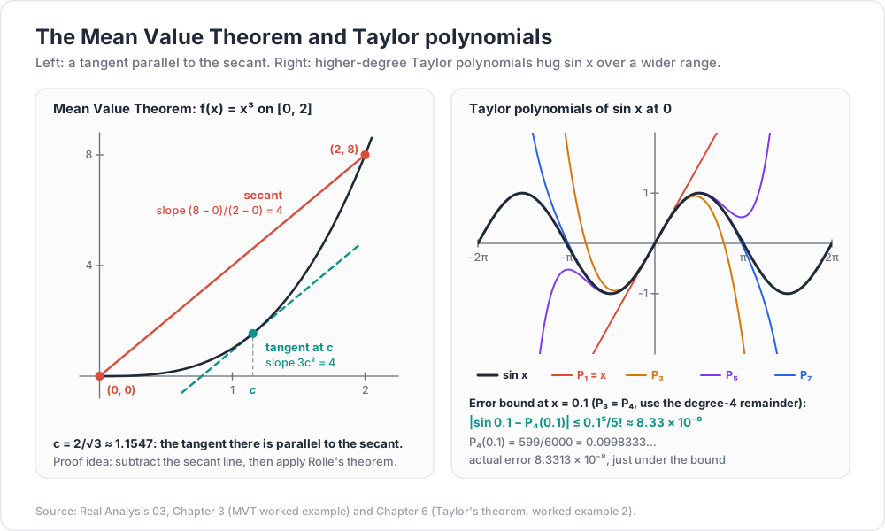
Geometrically: somewhere the tangent line is parallel to the secant line through the end points.

Proof. Subtract the secant line. Let

$$h(x) = f(x) - \left( f(a) + \frac{f(b) - f(a)}{b - a}\,(x - a) \right).$$

Then $h$ is continuous on $[a, b]$, differentiable on $(a, b)$, and $h(a) = h(b) = 0$. Rolle gives $c \in (a, b)$ with $0 = h'(c) = f'(c) - \frac{f(b) - f(a)}{b - a}$. $\blacksquare$

Worked example. $f(x) = x^3$ on $[0, 2]$. The secant slope is $\frac{8 - 0}{2 - 0} = 4$. Solve $f'(c) = 3c^2 = 4$ in $(0, 2)$: $c = \frac{2}{\sqrt 3} \approx 1.1547$. The theorem only promises that such a $c$ exists; here you can find it.

Consequences

Corollary 1 (zero derivative). If $f'(x) = 0$ for every $x$ in an interval $I$, then $f$ is constant on $I$.

Proof. Take $x < y$ in $I$. The MVT on $[x, y]$ gives $f(y) - f(x) = f'(c)(y - x) = 0$. $\blacksquare$

The interval matters: $f(x) = \operatorname{sign}(x)$ on $\mathbb{R} \setminus \{0\}$ has $f' = 0$ everywhere on its domain but is not constant, because the domain is not an interval.

Corollary 2 (same derivative). If $f' = g'$ on an interval, then $f - g$ is constant. This is why antiderivatives are unique "up to $+C$".

Corollary 3 (monotonicity). On an interval $I$, with $f$ differentiable on $I$:

Hypothesis on the interval	Conclusion
$f' \geq 0$	$f$ is increasing ($x < y \Rightarrow f(x) \leq f(y)$)
$f' > 0$	$f$ is strictly increasing
$f' \leq 0$ or $f' < 0$	decreasing or strictly decreasing
$\lvert f'\rvert \leq M$	$\lvert f(x) - f(y)\rvert \leq M\lvert x - y\rvert$ (Lipschitz)

Each line is one application of $f(y) - f(x) = f'(c)(y - x)$. The converse of line 2 fails: $x^3$ is strictly increasing but $f'(0) = 0$.

Worked example: a Lipschitz bound. Since $\lvert \cos\rvert \leq 1$, the last line gives $\lvert \sin a - \sin b\rvert \leq \lvert a - b\rvert$ for all real $a, b$.

Worked example: estimating a square root. Apply the MVT to $\sqrt{x}$ on $[100, 101]$: $\sqrt{101} - 10 = \frac{1}{2\sqrt c}$ for some $c \in (100, 101)$. Since $10 < \sqrt c < \sqrt{101}$,

$$0.04975\ldots = \frac{1}{2\sqrt{101}} < \sqrt{101} - 10 < \frac{1}{20} = 0.05.$$

The true value is $\sqrt{101} - 10 = 0.049875\ldots$, inside the bracket.

Cauchy's generalised Mean Value Theorem

Theorem (Cauchy MVT). Let $f, g$ be continuous on $[a, b]$ and differentiable on $(a, b)$. Then there is $c \in (a, b)$ with

$$\bigl(f(b) - f(a)\bigr)\,g'(c) = \bigl(g(b) - g(a)\bigr)\,f'(c).$$

Proof. Let $h(x) = \bigl(f(b) - f(a)\bigr) g(x) - \bigl(g(b) - g(a)\bigr) f(x)$. A direct computation gives $h(a) = f(b)g(a) - g(b)f(a) = h(b)$. Rolle gives $c$ with $h'(c) = 0$, which is the claim. $\blacksquare$

With $g(x) = x$ this is the ordinary MVT. The version with two functions is what L'Hôpital's rule needs.

---

Chapter 4 — Derivatives are not arbitrary functions

A derivative that is not continuous

Let

$$g(x) = \begin{cases} x^2 \sin(1/x) & x \neq 0, \\ 0 & x = 0. \end{cases}$$

At $0$: $\left\lvert \frac{g(x) - g(0)}{x} \right\rvert = \lvert x \sin(1/x)\rvert \leq \lvert x\rvert \to 0$, so $g'(0) = 0$. For $x \neq 0$ the ordinary rules give

$$g'(x) = 2x\sin(1/x) - \cos(1/x).$$

As $x \to 0$ the first term tends to $0$ but $\cos(1/x)$ oscillates between $-1$ and $1$ for ever. So $g'$ exists at every point of $\mathbb{R}$, yet $\lim_{x \to 0} g'(x)$ does not exist. A function can be differentiable everywhere with a discontinuous derivative. In the notation of Chapter 1: $g$ is differentiable on $\mathbb{R}$ but $g \notin C^1(\mathbb{R})$.

Darboux's theorem

Discontinuous derivatives still cannot jump. They always have the intermediate value property.

Theorem (Darboux). Let $f$ be differentiable on $[a, b]$ (one-sided at the endpoints). If $y$ lies strictly between $f'(a)$ and $f'(b)$, then there is $c \in (a, b)$ with $f'(c) = y$.

Proof. Assume $f'(a) < y < f'(b)$ (the other case is symmetric). Let $g(x) = f(x) - yx$. Then $g$ is differentiable on $[a, b]$ with $g'(a) = f'(a) - y < 0$ and $g'(b) = f'(b) - y > 0$. As a continuous function on $[a, b]$, $g$ attains a minimum at some $c$ (EVT).

• $c \neq a$: since $g'(a) < 0$, the quotient $\frac{g(x) - g(a)}{x - a}$ is negative for $x$ slightly bigger than $a$, so $g(x) < g(a)$ there, and $a$ is not a minimum.
• $c \neq b$: since $g'(b) > 0$, the quotient $\frac{g(x) - g(b)}{x - b}$ is positive for $x$ slightly smaller than $b$; the denominator is negative, so $g(x) < g(b)$, and $b$ is not a minimum.

So $c \in (a, b)$ and the interior extremum theorem gives $g'(c) = 0$, that is, $f'(c) = y$. $\blacksquare$

Note that the proof does not use the Intermediate Value Theorem for $f'$, because $f'$ need not be continuous.

Consequence. A derivative cannot have a jump discontinuity. For example, there is no differentiable $F : \mathbb{R} \to \mathbb{R}$ with $F'(x) = \operatorname{sign}(x)$ for all $x$: that function takes the values $-1$ and $1$ but never $\tfrac12$.

Common pitfall: "has the intermediate value property" does not imply "continuous". The derivative $g'$ above has the property (by Darboux) and is discontinuous at $0$.

---

Chapter 5 — L'Hôpital's rule

Theorem (L'Hôpital, zero-over-zero form). Let $f, g$ be differentiable on $(a, b)$, with $g'(x) \neq 0$ for all $x \in (a, b)$. Suppose

$$\lim_{x \to a^+} f(x) = 0, \qquad \lim_{x \to a^+} g(x) = 0, \qquad \lim_{x \to a^+} \frac{f'(x)}{g'(x)} = L,$$

where $L \in \mathbb{R}$ (the rule also holds for $L = \pm\infty$). Then $\lim_{x \to a^+} \frac{f(x)}{g(x)} = L$. The same holds for $x \to b^-$, for two-sided limits, and for $x \to \pm\infty$.

Proof ($L$ finite). Extend $f$ and $g$ to $[a, b)$ by $f(a) = g(a) = 0$; they are now continuous on $[a, x]$ for each $x \in (a, b)$. By Rolle, $g(x) \neq 0$ (otherwise $g' = 0$ somewhere in $(a, x)$). Cauchy's MVT on $[a, x]$ gives $c_x \in (a, x)$ with

$$\frac{f(x)}{g(x)} = \frac{f(x) - f(a)}{g(x) - g(a)} = \frac{f'(c_x)}{g'(c_x)}.$$

Given $\varepsilon > 0$, choose $\delta$ with $\left\lvert \frac{f'(t)}{g'(t)} - L \right\rvert < \varepsilon$ for $a < t < a + \delta$. If $a < x < a + \delta$ then $a < c_x < a + \delta$ too, so $\left\lvert \frac{f(x)}{g(x)} - L\right\rvert < \varepsilon$. $\blacksquare$

The infinity-over-infinity form. The same conclusion holds if instead $\lim_{x \to a^+} \lvert g(x)\rvert = \infty$ (nothing more is needed about $f$). The proof is a little longer; see Rudin, Theorem 5.13.

Worked example. Find $\lim_{x \to 0} \frac{x - \sin x}{x^3}$.

1. $f(x) = x - \sin x$ and $g(x) = x^3$ both tend to $0$; the quotient of derivatives is $\frac{1 - \cos x}{3x^2}$, still of the form $0/0$.
2. Differentiate again: $\frac{\sin x}{6x}$, still $0/0$.
3. Once more: $\frac{\cos x}{6} \to \frac16$.

Reading the chain backwards, each step's hypotheses hold near $0$: the denominators $x^3$, $3x^2$, $6x$ have derivatives $3x^2$, $6x$, $6$, which are non-zero for $x \neq 0$. So

$$\lim_{x \to 0} \frac{x - \sin x}{x^3} = \frac16.$$

Common pitfall: the rule goes one way only. With $f(x) = x + \sin x$ and $g(x) = x$ as $x \to \infty$, $f/g = 1 + \frac{\sin x}{x} \to 1$, but $f'/g' = 1 + \cos x$ has no limit. The rule is silent, not wrong: its hypothesis "the limit of $f'/g'$ exists" fails.

Watch out: check the $0/0$ or $\infty/\infty$ form first. $\lim_{x \to 0} \frac{x + 1}{x + 2} = \frac12$, but "differentiating" top and bottom gives $1$.

---

Chapter 6 — Taylor's theorem

Taylor polynomials

If $f$ is $n$ times differentiable at $a$, its Taylor polynomial of degree $n$ at $a$ is

$$P_n(x) = \sum_{k=0}^{n} \frac{f^{(k)}(a)}{k!}(x - a)^k = f(a) + f'(a)(x - a) + \dots + \frac{f^{(n)}(a)}{n!}(x - a)^n.$$

It is the unique polynomial of degree at most $n$ whose value and first $n$ derivatives at $a$ match those of $f$. $P_1$ is the tangent line. The remainder is $R_n(x) = f(x) - P_n(x)$. Everything useful about Taylor polynomials is a statement about $R_n$.

The theorem

Theorem (Taylor, Lagrange remainder). Let $n \geq 0$. Suppose $f^{(n)}$ is continuous on $[a, b]$ and differentiable on $(a, b)$. Then there is $c \in (a, b)$ with

$$f(b) = \sum_{k=0}^{n} \frac{f^{(k)}(a)}{k!}(b - a)^k + \frac{f^{(n+1)}(c)}{(n+1)!}(b - a)^{n+1}.$$

The same holds with $b < a$ (then $c$ lies between $b$ and $a$). For $n = 0$ this is exactly the MVT.

Proof. Let $P_n$ be the Taylor polynomial at $a$ and choose the number $M$ so that

$$f(b) = P_n(b) + M(b - a)^{n+1}.$$

Define $g(x) = f(x) - P_n(x) - M(x - a)^{n+1}$ on $[a, b]$. Because $P_n^{(k)}(a) = f^{(k)}(a)$ for $k \leq n$ and every derivative of order at most $n$ of $(x-a)^{n+1}$ vanishes at $a$,

$$g(a) = g'(a) = \dots = g^{(n)}(a) = 0, \qquad g(b) = 0.$$

• Rolle on $[a, b]$ with $g(a) = g(b) = 0$ gives $x_1 \in (a, b)$ with $g'(x_1) = 0$.
• Rolle on $[a, x_1]$ with $g'(a) = g'(x_1) = 0$ gives $x_2 \in (a, x_1)$ with $g''(x_2) = 0$.
• Continue: after $n + 1$ steps you have $x_{n+1} \in (a, b)$ with $g^{(n+1)}(x_{n+1}) = 0$.

(The hypotheses let each step apply Rolle: $g^{(k)}$ is continuous on $[a, b]$ and differentiable on $(a, b)$ for every $k \leq n$.) Since $P_n$ has degree at most $n$, $P_n^{(n+1)} = 0$, and the $(n+1)$-th derivative of $M(x - a)^{n+1}$ is $(n+1)!\,M$. So $0 = f^{(n+1)}(x_{n+1}) - (n+1)!\,M$. With $c = x_{n+1}$, $M = \frac{f^{(n+1)}(c)}{(n+1)!}$, which is the claim. $\blacksquare$

The error bound you actually use. If $\lvert f^{(n+1)}(t)\rvert \leq K$ for all $t$ between $a$ and $x$, then

$$\lvert f(x) - P_n(x)\rvert \leq \frac{K}{(n+1)!}\,\lvert x - a\rvert^{n+1}.$$

Worked example 1: the number e

Take $f(x) = e^x$, $a = 0$, $x = 1$. Every derivative is $e^x$, so $P_n(1) = \sum_{k=0}^{n} \frac{1}{k!}$ and

$$e - P_n(1) = \frac{e^{c}}{(n+1)!} \quad \text{for some } c \in (0, 1).$$

You also need a bound on $e$ that does not use this computation. The standard one is $e < 3$: expanding $(1 + 1/m)^m$ with the binomial theorem shows that every term of the sequence defining $e$ is at most $\sum_{k=0}^{m} \frac{1}{k!}$, and since $k! \geq 2^{k-1}$ this is at most $1 + 1 + \tfrac12 + \tfrac16 + \bigl(\tfrac18 + \tfrac1{16} + \dots\bigr) = \tfrac{35}{12} < 3$. With $e^c < e < 3$ you get $0 < e - P_n(1) < \frac{3}{(n+1)!}$.

With $n = 7$:

$$P_7(1) = 1 + 1 + \tfrac12 + \tfrac16 + \tfrac1{24} + \tfrac1{120} + \tfrac1{720} + \tfrac1{5040} = \frac{685}{252} = 2.718253968\ldots,$$

and the error is below $\frac{3}{8!} = \frac{3}{40320} \approx 7.44 \times 10^{-5}$. The true error is $e - \frac{685}{252} \approx 2.79 \times 10^{-5}$, inside the bound. The bound is honest: it is proved, not observed.

Worked example 2: sin(0.1) with an almost sharp bound

For $f = \sin$ at $a = 0$ the derivatives cycle through $\sin, \cos, -\sin, -\cos$, so

$$\sin x = x - \frac{x^3}{3!} + \frac{x^5}{5!} - \frac{x^7}{7!} + \dots$$

The coefficient of $x^4$ is $0$, so $P_3 = P_4$. Use the degree-4 remainder, which involves $f^{(5)} = \cos$ with $\lvert\cos\rvert \leq 1$:

$$\lvert \sin(0.1) - P_4(0.1)\rvert \leq \frac{(0.1)^5}{5!} = \frac{10^{-5}}{120} \approx 8.33 \times 10^{-8}.$$

Here $P_4(0.1) = 0.1 - \frac{0.001}{6} = \frac{599}{6000} = 0.0998333\ldots$, while $\sin(0.1) = 0.0998334166\ldots$. The actual error is $8.3313 \times 10^{-8}$, just under the bound $8.3333 \times 10^{-8}$.

Trick: when the next Taylor coefficient is zero, the degree-$n$ polynomial equals the degree-$(n+1)$ one, and you may use the smaller, higher-order remainder. For $\sin$ and $\cos$ this gains a whole power of $x$ for free.

Watch out: the bound needs $K$ to bound $f^{(n+1)}$ on the whole interval between $a$ and $x$, not just at $a$. For $e^x$ on $[0, 1]$ that is why you need $e < 3$ first.

---

Chapter 7 — Smooth, analytic, and the monsters

Smooth but not analytic

Let

$$f(x) = \begin{cases} e^{-1/x^2} & x \neq 0, \\ 0 & x = 0. \end{cases}$$

Claim. $f$ is $C^\infty$ on $\mathbb{R}$ and $f^{(k)}(0) = 0$ for every $k \geq 0$.

Sketch of proof. For $x \neq 0$, induction shows $f^{(k)}(x) = p_k(1/x)\,e^{-1/x^2}$ for some polynomial $p_k$. At $0$, use the definition and induction: $\frac{f^{(k)}(x) - 0}{x} = \frac1x p_k(1/x) e^{-1/x^2}$, and with $t = 1/x$ this is a polynomial in $t$ times $e^{-t^2}$, which tends to $0$ as $\lvert t\rvert \to \infty$ because $e^{t^2}$ outgrows every power of $t$. So $f^{(k+1)}(0) = 0$. $\blacksquare$

Consequently every Taylor polynomial of $f$ at $0$ is the zero polynomial, and $R_n(x) = f(x) > 0$ for every $x \neq 0$ and every $n$. The Taylor series at $0$ converges everywhere, to the wrong function. So "infinitely differentiable" does not imply "equal to its Taylor series". A function that equals its Taylor series near each point is called (real) analytic; this $f$ is smooth but not analytic at $0$. Taylor's theorem is not wrong here: it only claims the remainder has the Lagrange form, and here the remainder simply does not go to $0$. Post 05 returns to this with power series.

Continuous but nowhere differentiable

Theorem (Weierstrass, 1872). Let $0 < a < 1$, let $b$ be an odd positive integer, and let $ab > 1 + \frac{3\pi}{2}$. Then

$$W(x) = \sum_{n=0}^{\infty} a^n \cos(b^n \pi x)$$

is continuous at every $x \in \mathbb{R}$ and differentiable at no $x \in \mathbb{R}$.

For example, $a = \frac12$, $b = 13$ gives $ab = 6.5 > 1 + \frac{3\pi}{2} \approx 5.712$. Continuity comes from the Weierstrass M-test of post 05: $\lvert a^n \cos(b^n \pi x)\rvert \leq a^n$ and $\sum a^n$ converges, so the series converges uniformly, and uniform limits of continuous functions are continuous. The non-differentiability proof is a careful estimate of difference quotients (Hardy showed in 1916 that $ab \geq 1$ is enough). The picture to keep: the graph has corners at every scale, like $\lvert x\rvert$ at $0$, but everywhere.

The hierarchy

Class	Example that is in this class but not the next
continuous	$\lvert x\rvert$ (not differentiable at 0)
differentiable	$x^2\sin(1/x)$ (derivative not continuous at 0)
$C^1$	$x\lvert x\rvert$ (derivative $2\lvert x\rvert$, not differentiable at 0)
$C^\infty$	$e^{-1/x^2}$ (not analytic at 0)
analytic	$\sin x$, $e^x$, polynomials

Each row is strictly larger than the next. Weierstrass's $W$ sits in row 1 and is as far from row 2 as possible.

---

Practice Exercises

Exercise 1. Show that $f(x) = x\lvert x\rvert$ is differentiable on $\mathbb{R}$ with $f'(x) = 2\lvert x\rvert$, and that $f'$ is not differentiable at $0$.

Solution

For $x > 0$, $f(x) = x^2$ so $f'(x) = 2x$; for $x < 0$, $f(x) = -x^2$ so $f'(x) = -2x$. At $0$: $\frac{f(x) - f(0)}{x} = \lvert x\rvert \to 0$, so $f'(0) = 0$. In all cases $f'(x) = 2\lvert x\rvert$. Then $f' = 2\lvert x\rvert$ has a corner at $0$ (difference quotients $\pm 2$), so $f''(0)$ does not exist. So $f \in C^1(\mathbb{R})$ but $f$ is not twice differentiable.

Exercise 2. Find the point $c$ promised by the MVT for $f(x) = \sqrt{x}$ on $[1, 4]$.

Solution

Secant slope $\frac{\sqrt4 - \sqrt1}{4 - 1} = \frac13$. Solve $f'(c) = \frac{1}{2\sqrt c} = \frac13$: $\sqrt c = \frac32$, so $c = \frac94 = 2.25$, which lies in $(1, 4)$.

Exercise 3. Prove that $\ln(1 + x) < x$ for every $x > 0$.

Solution

Apply the MVT to $\ln(1 + t)$ on $[0, x]$: $\ln(1 + x) - \ln 1 = \frac{1}{1 + c}\,x$ for some $c \in (0, x)$. Since $c > 0$, $\frac{1}{1 + c} < 1$, so $\ln(1 + x) < x$.

Exercise 4. Compute $\lim_{x \to 0} \frac{1 - \cos x}{x^2}$ with L'Hôpital's rule, checking the hypotheses.

Solution

Both $1 - \cos x$ and $x^2$ tend to $0$, both are differentiable, and $(x^2)' = 2x \neq 0$ for $x \neq 0$. The quotient of derivatives is $\frac{\sin x}{2x} \to \frac12$ (using $\frac{\sin x}{x} \to 1$, or one more application of the rule). So the limit is $\frac12$.

Exercise 5. Approximate $\sqrt{1.1}$ by the degree-2 Taylor polynomial of $\sqrt{1 + x}$ at $0$, and prove an error bound.

Solution

$f(x) = (1 + x)^{1/2}$ gives $f(0) = 1$, $f'(0) = \frac12$, $f''(0) = -\frac14$, so $P_2(x) = 1 + \frac{x}{2} - \frac{x^2}{8}$ and $P_2(0.1) = 1 + 0.05 - 0.00125 = 1.04875$. The third derivative is $f'''(t) = \frac38 (1 + t)^{-5/2}$, which is at most $\frac38$ for $t \in (0, 0.1)$. So

$$\lvert \sqrt{1.1} - 1.04875\rvert \leq \frac{3/8}{3!}(0.1)^3 = \frac{1}{16000} = 6.25 \times 10^{-5}.$$

Check: $\sqrt{1.1} = 1.0488088\ldots$, an error of about $5.88 \times 10^{-5}$. Since $f''' > 0$ the remainder is positive, so $1.04875$ is an underestimate.

Exercise 6. Suppose $f : \mathbb{R} \to \mathbb{R}$ satisfies $\lvert f(x) - f(y)\rvert \leq (x - y)^2$ for all $x, y$. Prove that $f$ is constant.

Solution

For $x \neq y$, $\left\lvert \frac{f(x) - f(y)}{x - y}\right\rvert \leq \lvert x - y\rvert$. Letting $x \to y$ gives $f'(y) = 0$ for every $y$. By Corollary 1 of the MVT on the interval $\mathbb{R}$, $f$ is constant.

Exercise 7. Can the floor function $\lfloor x \rfloor$ be the derivative of some function $F$ on $[0, 2]$?

Solution

No. On $[0, 2]$ the floor function takes the values $0$, $1$ and $2$ but never $\frac12$. If $F' = \lfloor x \rfloor$ on $[0, 2]$, Darboux's theorem on $[0, 1]$ (where $F'(0) = 0$ and $F'(1) = 1$) would give $c$ with $F'(c) = \frac12$. Contradiction.

---

Cheat-sheet

Result	Hypotheses	Conclusion
Differentiable ⇒ continuous	$f'(c)$ exists	$f$ continuous at $c$
Carathéodory form	$f'(c)$ exists	$f(x) - f(c) = \varphi(x)(x - c)$, $\varphi$ continuous at $c$
Chain rule	$g'(c)$ and $f'(g(c))$ exist	$(f\circ g)'(c) = f'(g(c))g'(c)$
Interior extremum	max or min at interior $c$, $f'(c)$ exists	$f'(c) = 0$
Rolle	continuous on $[a,b]$, diff. on $(a,b)$, $f(a) = f(b)$	some $f'(c) = 0$
MVT	continuous on $[a,b]$, diff. on $(a,b)$	$f(b) - f(a) = f'(c)(b - a)$
Cauchy MVT	same, for $f$ and $g$	$(f(b) - f(a))g'(c) = (g(b) - g(a))f'(c)$
Darboux	diff. on $[a,b]$	$f'$ has the intermediate value property
L'Hôpital	$0/0$ or $\infty/\infty$, $g' \neq 0$, $f'/g' \to L$	$f/g \to L$
Taylor (Lagrange)	$f^{(n)}$ continuous on $[a,b]$, diff. on $(a,b)$	$R_n = \frac{f^{(n+1)}(c)}{(n+1)!}(b - a)^{n+1}$
Error bound	$\lvert f^{(n+1)}\rvert \leq K$ between $a$ and $x$	$\lvert R_n(x)\rvert \leq \frac{K}{(n+1)!}\lvert x - a\rvert^{n+1}$
Smooth but not analytic	$e^{-1/x^2}$	all $f^{(k)}(0) = 0$, Taylor series is $0$

---

What's next

Post 04 builds the Riemann integral from scratch: partitions, upper and lower Darboux sums, the Riemann criterion, and proofs that continuous and monotone functions are integrable. The Mean Value Theorem from this post is the engine of the proof of the Fundamental Theorem of Calculus there, and a relative of $x^2\sin(1/x)$ returns as a warning about what that theorem needs.

---

References

• Stephen Abbott, Understanding Analysis, 2nd ed., Springer (Undergraduate Texts in Mathematics), 2015 — Chapter 5, "The Derivative", including Darboux's theorem and a continuous nowhere-differentiable function.
• Walter Rudin, Principles of Mathematical Analysis, 3rd ed., McGraw-Hill, 1976 — Chapter 5 (Theorems 5.10 MVT, 5.12 Darboux, 5.13 L'Hôpital, 5.15 Taylor).
• Robert G. Bartle and Donald R. Sherbert, Introduction to Real Analysis, 4th ed., Wiley, 2011 — Chapter 6, including the Carathéodory form of the chain rule.
• Michael Spivak, Calculus, 4th ed., Publish or Perish, 2008 — Chapters 10–11 and 20 (Taylor polynomials and remainders).
• Jiří Lebl, Basic Analysis I: Introduction to Real Analysis, free textbook — jirka.org/ra, Chapter 4.
• MIT OpenCourseWare, 18.100A Real Analysis (Fall 2020), lecture notes on differentiation and Taylor's theorem.
• G. H. Hardy, "Weierstrass's non-differentiable function", Transactions of the American Mathematical Society 17 (1916), 301–325.

Note: this post is in progress. Planned additions: the Peano and integral forms of the Taylor remainder, convex functions and the second-derivative test, a full proof that the Weierstrass function is nowhere differentiable, and Newton's method with its quadratic error bound.